Lecture 35: STEP and drawings

A kernel is not done when it can build a shape. It has to take shapes in from other systems, and it has to put them out in forms people use: a drawing for a machinist, a mesh for a printer or a screen. All three of those are translations between what the kernel knows, and formats that know less or differently. This lecture is about what such a translation keeps, and what it must be honest about losing.

STEP

STEP (ISO 10303) is the standard neutral format for exchanging B-reps. A file is plain text in the encoding of Part 21: a header, then a data section of numbered entity instances. An application protocol says which entities are meaningful: AP203, AP214 and AP242 are the ones you meet for mechanical parts, and they share the B-rep geometry.

Here is the top of a real file, written by the kernel: geop compile of the example rounded_box, to .step, with most lines elided as ....

ISO-10303-21;
HEADER;
FILE_DESCRIPTION(('rounded_box'),'2;1');
FILE_NAME('rounded_box.step','',(''),(''),'geop','geop','');
FILE_SCHEMA(('AUTOMOTIVE_DESIGN { 1 0 10303 214 1 1 1 1 }'));
ENDSEC;
DATA;
#1=APPLICATION_CONTEXT('core data for automotive mechanical design processes');
...
#3=(LENGTH_UNIT() NAMED_UNIT(*) SI_UNIT(.MILLI.,.METRE.));
...
#6=UNCERTAINTY_MEASURE_WITH_UNIT(LENGTH_MEASURE(1.E-7),#3,'distance_accuracy_value','confusion accuracy');
...
#8=CARTESIAN_POINT('',(0.2,0.2,-2.7755575615628914E-17));
...
#688=CLOSED_SHELL('',(#47,#87,#125,...));
#689=MANIFOLD_SOLID_BREP('fillet(round)',#688);

The entities form a graph by # reference. From the solid down:

MANIFOLD_SOLID_BREP → CLOSED_SHELL → ADVANCED_FACE → FACE_OUTER_BOUND → EDGE_LOOP
   → ORIENTED_EDGE → EDGE_CURVE → VERTEX_POINT → CARTESIAN_POINT
                         ↳ the edge's curve        ADVANCED_FACE ↳ its surface

That maps almost one to one onto Lecture 17’s model: ORIENTED_EDGE is a coedge, EDGE_CURVE an edge. The file above has 26 ADVANCED_FACEs, 48 EDGE_CURVEs and 24 VERTEX_POINTs, and $24-48+26=2$, as Euler requires for a solid with no holes. (6 flat faces, 12 fillets, 8 corner patches.) Look at what is not there: a pcurve. A STEP edge has a 3-D curve and may or may not have pcurves (SURFACE_CURVE, in the larger entity set). Geop requires them for every coedge, so the importer has to make them.

A complex instance such as #3=(LENGTH_UNIT() NAMED_UNIT(*) SI_UNIT(...)) is a single instance of several entity types at once. ops/geop-ops-step/src/part21.rs reads the encoding and knows nothing of what the entities mean; meaning belongs to ops/geop-ops-step/src/import/ and ops/geop-ops-step/src/export.rs.

Reading: three differences to bridge

import/structure.rs finds the bodies: every MANIFOLD_SOLID_BREP, BREP_WITH_VOIDS and SHELL_BASED_SURFACE_MODEL, with their units, and in an assembly walks down from the products nothing places, composing placements (through NEXT_ASSEMBLY_USAGE_OCCURRENCE and ITEM_DEFINED_TRANSFORMATION) into one per body. import/geometry.rs reads curves and surfaces. import/body.rs, at 3700 lines the largest file of the crate, reads the topology. Its opening comment lists the three ways a STEP B-rep and a Geop one differ.

Everything becomes NURBS. A file has PLANE, CYLINDRICAL_SURFACE, CONICAL_SURFACE, SPHERICAL_SURFACE, TOROIDAL_SURFACE, SURFACE_OF_REVOLUTION, SURFACE_OF_LINEAR_EXTRUSION, B_SPLINE_SURFACE, and LINE, CIRCLE, ELLIPSE. Each analytic type is built as an exact NURBS covering its face (Lecture 8), and a B-spline is taken as it is. The kernel’s “no branch on surface kinds” begins where the data comes in: this importer’s dispatch on the entity’s type is the only place the type matters, and it vanishes right after.

The file is read into plain f64 definitions (CurveDef, SurfaceDef), used for decisions such as where a face wraps and which loop is outer: “it is data, decided on before anything exact is built from it”.

Periodic surfaces. STEP parametrizes a cylinder all the way round, so a face going round its axis runs along a seam, one edge its loop uses twice, or is bounded by loops that go once round each. A Geop surface is a patch that does not wrap: its loops close in $(u,v)$ (Lecture 18). So a wrapping face is cut along meridians into sectors, each on a patch of its own: Builder::cut_wrapping_face. A face going round a torus’s tube is cut along parallels (Builder::cut_tube_wrapping_face), and a whole torus into bands first (Builder::cut_whole_torus). A thread’s flank, which turns more than once without going round, is cut along meridians too (Builder::cut_helical_face). The operation’s doc names the new pieces (fN,qM and so on), so a later step can refer to them.

Closed edges. A STEP edge may start and end at one vertex, a whole circle. A Geop edge may not, so it is split in two.

Then every pcurve is fitted by projecting the edge onto the surface, by NurbSurface::fit_pcurve (Lecture 16), the way all pcurves of the kernel are.

Reading: tolerance

A file’s numbers do not agree with each other. A vertex’s CARTESIAN_POINT, the ends of its edges’ curves, and the surfaces it should lie on, each say something slightly different, and the file’s UNCERTAINTY_MEASURE_WITH_UNIT says by how much that is allowed. A kernel can read a tolerance from the file and carry it beside the geometry. In Geop, every value already is an enclosure, so a file’s disagreement has somewhere natural to go.

A vertex is the union of every place the file says it is: its point, the ends of its edges’ curves, and its foot points on its faces’ surfaces. Union, because these are enclosures of one point that disagree, and the rule of Lecture 5 is to cover both. Its width is then an honest measure of how much the file disagrees with itself.

An edge is widened until it reaches the midpoints of its pcurve’s points on each of its faces, measured and widened in rounds: the first round by the file’s disagreement, later ones by rounding. There is a nice piece of honesty in that loop. Widening by exactly the gap left falls short by a rounding, and a comment records it: an edge 4.4e-16 off a plane “was widened four times and ended 6.7e-80 short of it”. So later rounds widen by twice the gap, and the comment says this is “a workaround, kept knowingly”, giving what the fix would be.

What lies further apart than the kernel can carry is rebuilt. The limit is ACCURACY, 1e-4: the widest a vertex or a control point may be (Lecture 20). Past that, heal rebuilds from the surfaces, since a B-rep is defined by them: a vertex where its faces’ surfaces meet, an edge along where they meet. Where the surfaces themselves contradict each other, the smallest faces there are left out, and rebuilt from their edges (rebuilt_surface). The file’s uncertainty bounds this: what is rebuilt must lie on its surfaces to within it, and what cannot be is refused by name, as is anything that would move further than half the length of an edge there. What was rebuilt is reported as a Healing, with how far each thing moved, and shown to the user: a list of what the kernel changed, not a silent fix.

A trap at the last bit

Lecture 11 explains why curves evaluate relative to a control point of the span. A STEP file showed the other side of it. An edge lay 2e-31 above its plane face (AGENTS.md, Evaluate relative to the patch). Evaluated relative to a control point 1.8e-15 up, its enclosure took in the plane, because the relative evaluation adds that point back with one rounding, and an ulp at 1.8e-15 is about 4e-31. So the importer measured no gap and did not widen the edge. Validation’s clipping, which reads control points, found the face’s points off it.

Neither computation was wrong. Each is a true enclosure, and each is the tighter one somewhere. So NurbCurve::evaluate (core/geop-core-geometry/src/nurb_curve/evaluate.rs) computes both, absolute and relative, and intersects them. Two enclosures of one value with different numerical strengths: their intersection is still a true enclosure. That rule is from Lecture 5, and it took a real file’s 2e-31 to need it.

Writing, and the corpus

Writing is far simpler (ops/geop-ops-step/src/export.rs, write_step, write_part): each solid a MANIFOLD_SOLID_BREP, each sheet a SHELL_BASED_SURFACE_MODEL, every surface and curve “written exactly as the kernel holds it: a B_SPLINE_*_WITH_KNOTS, rational where a weight is not one”. The file above reflects this: it holds not one CYLINDRICAL_SURFACE. Another system receives correct B-splines, not recognisable primitives; a cylinder comes back as a spline to it. Values are written as interval midpoints: a format with no enclosures can only hold a number. Names of entities are the part’s own ('fillet(round)' above). An assembly becomes products and occurrences.

Testing an importer against files you made yourself proves little, since real files come from other kernels’ idiosyncrasies. ops/geop-ops-step/scripts/fetch_corpus.sh downloads public files, the NIST MBE PMI test models, STEP files from the OCCT, CadQuery and build123d repositories, and a spread of the FreeCAD parts library, into target/step-corpus/, never committed. The ignored test corpus (ops/geop-ops-step/src/corpus.rs) imports them all, validates them, and prints a table of what passed and why the rest failed, with STEP_CORPUS_ONLY and STEP_CORPUS_FULL to narrow or deepen it. We did not run it for this book, so no pass rate is quoted here.

STL

The other way in is a mesh. ImportStl (ops/geop-ops-step/src/stl.rs) reads either form of STL, makes each triangle a face with BodySpec::of_triangles, and merges coplanar triangles into one face with BodySpec::merged. A solid if every edge is shared by two triangles, a sheet otherwise. A mesh has no curved surfaces to recover, and it does not try to.

Drawings

An engineering drawing is a set of 2-D projections with visible lines solid and hidden lines dashed, on a sheet, with dimensions and a title block. It was the original CAD output, and it remains a contract: a machinist builds what the drawing says.

The following is a real sheet, written by the kernel with geop compile box_with_drill_hole.geop -o box_with_drill_hole.svg. In third-angle layout: the top view above the front view, the right view beside it, an isometric view at the upper right. The blind hole’s wall and floor are dashed wherever material hides them.

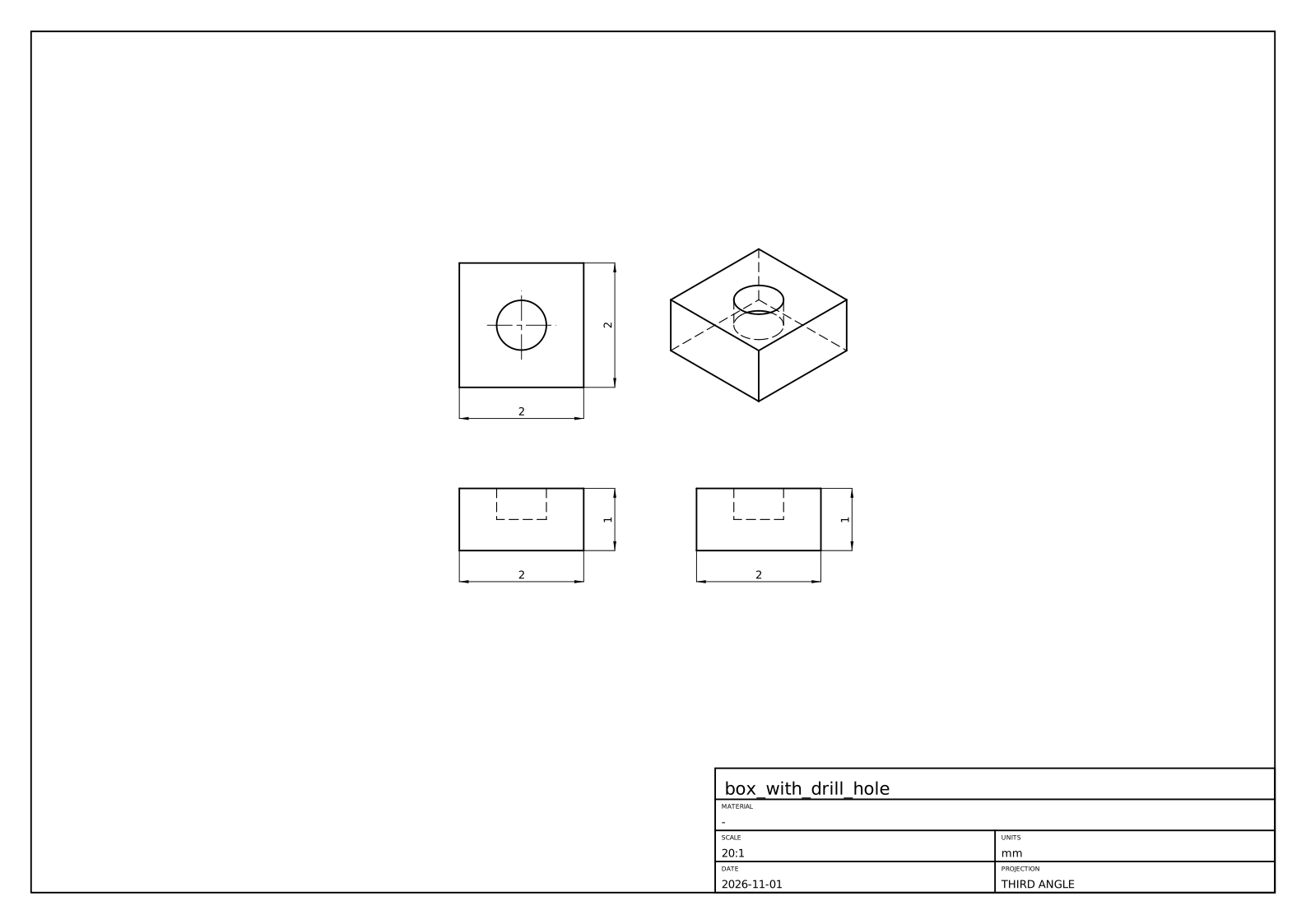
The crate is ops/geop-ops-drawing. Views come from ops/geop-ops-drawing/src/view.rs: “the views are the usual ones of a z-up modeller”. Let us look at how such lines are found.

Hidden-line removal in three steps

What should a view draw? Edges where faces meet at an angle (tangent edges only if asked), and the silhouettes of curved faces. Along such a curve, what is in front of it changes only where its projection meets the projection of another curve, passing behind an edge or a silhouette, or where it turns back on itself. That one observation gives the algorithm (project_view in ops/geop-ops-drawing/src/hidden_lines.rs):

1. Project every curve, exactly. Orthographic projection is linear, so a NURBS curve projects to a NURBS curve with the same knots and weights (ViewFrame::project_curve).
2. Cut each one wherever its projection crosses or runs along another’s (curve_curve_overlaps_and_crossings), and wherever it is stationary along the paper’s axes (NurbCurve::stationary_parameters), which holds every point where it turns back.
3. One point decides a piece. Between cuts, nothing in front of it can change, so a ray from one point towards the eye gives the answer for the whole piece. If it crosses a face first, the piece is hidden.

This is sound, not a heuristic: step 2 removes every place where visibility could change. Look at what step 3 is doing in the context of “Do not decide from samples”: it takes one sample because the structure has proved the answer is constant along the piece. (That is the same shape of argument as Lecture 19 with faces and rays, and as a classification after remesh, Lecture 22.)

Three subtleties, all in seen:

• A crossing at the ray’s own start is no crossing: the point lies on the faces it bounds.
• A crossing on a face’s trim boundary means an edge is in front. The piece runs along that edge on the paper. So it is classified hidden, and a later pass (drop_drawn) drops it along with every piece lying on one already drawn. A hidden line under a visible one is never drawn, nor any line twice.
• A ray running in a face’s surface is seen edge-on, and “an edge-on face hides nothing”: curve_surface_overlaps catches it first.

Silhouettes

A cylinder seen from the side has two straight lines that are no edge. They are where the surface turns away from the eye. For a view along $d$, a point of the surface is on the silhouette when the normal is square to $d$:

$$g(u,v)=\bigl(S_u(u,v)\times S_v(u,v)\bigr)\cdot d=0.$$

This is a curve in $(u,v)$, and the kernel’s method (ops/geop-ops-drawing/src/silhouette.rs) is the one you know for an intersection (Lecture 16): a seed, then predictor-corrector steps along the tangent $(-g_v,g_u)$, then Newton back onto $g=0$.

Where do seeds come from? $g$’s sign is sampled along a grid of iso lines, with bisection between opposite signs. Is this a sample deciding an answer, against our rule? The comment is careful: “Sampling only decides where to look: what is traced is the exact zero set”. What could it miss, though? A closed loop crossing no grid line lies within one cell, and encloses a critical point of $g$, so each cell where $g$ could vanish is halved into boxes, those that could hold a critical point halved again, and a line through each is sampled too (loop_seats). The grid’s interior lines sit at irrational fractions of the domain, a free choice so they do not run along the symmetric iso lines silhouettes so often are.

Then each piece is trimmed against the face and fitted as a 3-D curve through exact silhouette points, widened to enclose what lies between (NurbCurve3D::fit_enclosing). The visibility test needs a point exactly on it, so it asks Silhouette::exact_point, since a ray grazing a face at its silhouette tells the truth only from the exact point.

A case: the duck’s ankle

A recent commit to this code (c0c70bb4) is a compact lesson in “Name the entities before you name the cause”, from AGENTS.md. Here is what its message records. The duck assembly, updated, did not draw from the right. A vague explanation is easy to imagine: a numerically awkward view. What it named instead: face 37 of the left ankle, the lower quarter cylinder of its D-shaped profile, extruded 15 along $x$; degree 1 along $x$, a rational quadratic round the arc. In the ankle’s frame, the right view looks along $(-1,-8.1\times10^{-15},3.9\times10^{-14})$: 4e-14 off the cylinder’s axis.

So $g$ was a rounding off zero all over the face. Is a silhouette there? Asked to the last bit, the check swept_along said this face is not swept along the view, and the tracer started. Its corrector returned the seed on the start edge at $v=[-50.8,105.5]$, in a domain of $[0,1]$: honest for a $g$ that noisy, but reaching past the domain, and the march then evaluated the arc there, where its weight could be zero.

Two fixes, each of which alone draws the duck. First, the question is asked at the right resolution. A drawing’s resolution is the sheet’s (COARSE_SUBDIVISION), and swept_along now decides to it: every control point of a row, of one weight, within it on the paper of the row’s first. The face then lies within it of the curve its first points span, which its edges draw, and so do its silhouettes. A generator seen 4e-14 off its length projects to a point. Second, the corrector cuts its answer to the domain: the silhouette sought is on the patch, and an interval argument is no licence to evaluate past it. The reproducer is quarter_cylinder_seen_a_hair_off_its_axis, which rebuilds face 37 from its enclosures.

Is the coarse decision an epsilon? It comes close to the line, so here is the reasoning as this book reads it. It does not decide whether a value of the geometry is zero; it decides whether a drawing, whose output is ink on paper, can see the difference, and the fallback when it says no is the edges, which draw the same ink. Compare is_point and the “sheet’s resolution” handoffs in seen. What must not depend on such a threshold is a claim about the geometry itself.

Assemblies, sections, and the sheet

An assembly places the same part a hundred times, and ops/geop-ops-drawing/src/scene.rs is built round that fact.

1. Each part on its own: a part’s lines and which of them its own faces hide, from a direction turned into its own frame. Placed parts of one component turned alike share this work.
2. The parts together (Scene::together): each line a part shows is cut where it crosses a line another part shows, each piece decided by a ray against that part’s faces.
3. Copies behind copies (Scene::mark_copies_behind): a copy exactly behind another adds no line, so a row of screws seen end on is drawn as one.

A stated limit: “A line is not cut where it enters another part, only where it passes behind its outline: parts that pierce each other are a known limit.”

A section view takes what lies on one side of a plane away, by the kernel’s own boolean: subtract a box standing on the plane from every solid (section_part in ops/geop-ops-drawing/src/section.rs); cut_faces finds what to hatch. No section code runs on its own: a section is a boolean plus the views above.

Then ops/geop-ops-drawing/src/drawing.rs composes: views laid out in third- or first-angle projection, centre marks on circles, overall sizes dimensioned, a border, a title block, and a parts list with balloons if asked for. An Annotation (a Distance, a Radius …) refers to what it measures by the entities’ names and the view’s, and its value is measured anew at each rebuild. “A drawing changes nothing, it only annotates.” It follows the part through every edit because it names things rather than storing positions.

Finally lib/geop-lib-sheet holds plain strokes and labels on layers, written by to_svg or to_dxf. Curves become lines, arcs and circles where they are those (NurbCurve3D::as_line, NurbCurve3D::as_arc), else polylines through points. This is one of the places “Where a user needs the exact line or arc back, as a sketch projecting an edge does, it is reconstructed locally where it is used” from AGENTS.md: the kernel holds a NURBS, and the DXF reader gets a true ARC.

The flat pattern’s DXF of Lecture 33 goes out the same way.

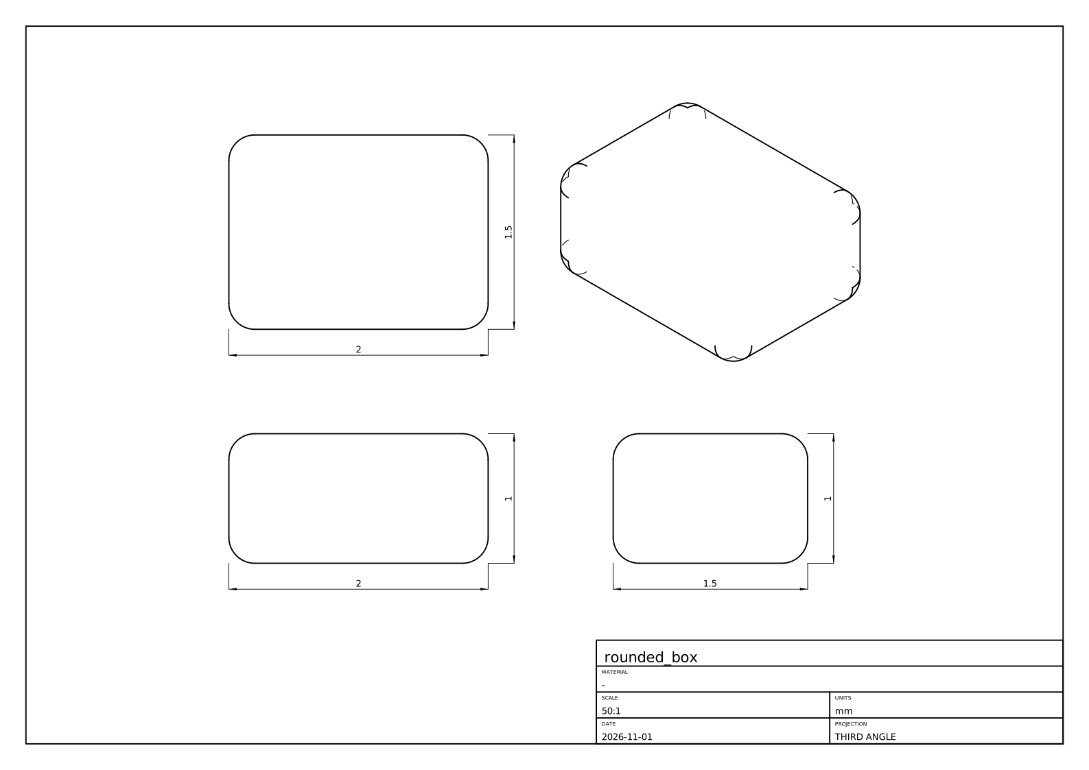
Here is a second real sheet, of rounded_box. Every outline in it is a silhouette: the fillets meet the flat faces tangentially, so the tangent edges are not drawn, and in the isometric view you can see the short silhouette arcs of the ball patches at the corners.

Meshes: the one place that samples

A screen and a 3-D printer want triangles. core/geop-core-rasterize turns a model into sampled geometry: a point per vertex, a polyline per edge, triangles per face, each tagged with the entity it came from, for drawing, picking, STL and debugging.

“Do not decide from samples” names this crate as its exception: “what it draws is a polygon, so sampling is what it is for”. So it is in plain f64, and its quality is a parameter that decides nothing but appearance. Being allowed to sample does not make it easy, though. The problems are combinatorial, not numeric.

The method (triangulate_face, core/geop-core-rasterize/src/grid.rs):

1. Every edge is sampled once (sample_curve), curvature-sized, and a face’s boundaries are placed in its $(u,v)$ from those samples, so two faces share exactly the same boundary points.
2. Pick a uniform $(u,v)$ grid: start from some $n$ and double until every cell’s flat approximation is within a curvature tolerance. A flat patch stays coarse, a curved one gets what it needs.
3. Split the outer boundary and each hole into convex parts, clip each to grid cells (clip_to_rect), subtract the holes’ parts in each cell (subtract_convex), and ear-clip what is left (ear_clip).

The module comment records three earlier versions that were wrong, a history worth reading: a slit from outer loop to hole that a cell boundary could cross; the same slit done per cell, with a visibility heuristic that could choose a wrong bridge; and clipping a concave outer boundary directly, which returned two pieces joined by a zero-width bridge, so that “a face whose trim went around a hole was drawn across it”. The version that stuck has no bridge to get wrong. A convex region is the intersection of its edges’ half planes, so its complement is the union of their outsides: peel off each outside part in turn.

Two traps

A mesh that ate the machine. AGENTS.md opens its rule “Cap every run’s memory and time” with this. A revolve that “crashed the boolean” was in fact the rasterizer: clipping a concave hole of many corners split it into exponentially many pieces, since subtract_convex kept degenerate leftovers. A concave hole is taken out as many triangles, one after another, and cutting every piece along every triangle’s sides whether it overlaps or not multiplies the pieces with each triangle. The fix is one test: if the leftover inside the hole is empty, the hole does not overlap the subject, and the subject is returned whole. Only interrupting a capped run under gdb showed where it was. The failure surfaced far from its cause, and looking only at the boolean would have found nothing.

A volume that weighed slivers. A closed mesh’s volume is $\sum_T\tfrac16\,a\cdot(b\times c)$, a sum of signed tetrahedra from the origin, by the divergence theorem. Each face was once sampled alone, so two faces met along a curved edge in two polygons a sliver apart: the mesh was not closed. The sum is exact only for a closed figure. Taken from the origin, those slivers were weighted by their distance from it: in a plate at $(10000,-5000,2000)$, AGENTS.md reports 5.5 of error for a bore of 142.

Two fixes, at two levels. enclosed_volume (core/geop-core-rasterize/src/stl.rs) takes its apex at a corner of the mesh, so “what is not closed weighs by its size”. And the mesh itself is now closed: core/geop-core-rasterize/src/mesh.rs makes it conforming, within a face (Mesh::conform) and across an edge (zip), every point any face put on an edge being put on it in every face that edge bounds, bit for bit. “An STL of a solid is a closed mesh.” Note that the mesh’s closure is combinatorial, enforced by construction, not by chance agreement of floats.

Note where exact volume comes from: not this mesh at all. Mass properties integrate the NURBS directly, by Green’s theorem, in core/geop-core-topology/src/mass.rs (Lecture 41). A mesh is for looking at.

Exercises

1. Verify Euler’s formula for the rounded_box STEP counts given above. Then predict $F,E,V$ for a box with one fillet on one edge, and for the same box with a through hole. (For a solid with one hole through it, $V-E+F=2-2g$ with $g$ the genus: but also note Geop requires a face with a hole to have two loops, so the formula needs the number of loops $L$.)

2. A file has a vertex whose point is $(1,0,0)$, an edge end at $(1+2\times10^{-7},0,0)$, and a foot on a surface at $(1-10^{-7},0,0)$. What enclosure does the importer build for the first coordinate, and what is its width? Is it accepted? How would your answer change if the edge end were at $1+3\times10^{-4}$?

3. In the hidden-line demo, choose “one box” and turn it to any general view. Count visible and hidden edges. Show that a convex polyhedron seen from a general direction shows an edge if and only if at least one adjacent face is front-facing. Why does the algorithm in the demo not need that rule, and what would it miss if it used only that?

4. Why must a curve be cut where its projection is stationary along the paper’s axes? Give an example of a curve that is seen wrongly if you cut only at crossings with other curves.

5. Find $g(u,v)$ for a cylinder of radius $R$ about the $z$ axis, with $S(u,v)=(R\cos u,R\sin u,v)$, viewed along $d=(d_x,d_y,d_z)$. Where is the silhouette? What happens as $d\to(0,0,1)$, and how does this relate to the duck’s ankle?

6. Suppose a mesh is not closed: there is a gap along a curved edge of length $\ell$ and width $\epsilon$. Estimate the volume error of the tetrahedra sum from an apex at distance $D$. Now take the numbers in the text, and check that $D\approx10^4$ and a sliver of area $\sim10^{-3}$ give the right order of error.