Building a CAD kernel
This book is a lecture series on how to build a modern CAD kernel. It starts from a linear algebra course and a little programming, and it ends with you able to read, debug and extend a real boundary-representation kernel: its intervals, its NURBS, its booleans, its sketch and assembly solvers, its fillets and shells, and the incremental build that runs them all.
The kernel it teaches is Geop, an open-source kernel in Rust. Every statement this book makes about the kernel is meant to hold against the code in this repository, and paths and function names are cited so that you can go and read them: core/geop-core-geometry/src/aabb.rs, compute_aabb. Where something is not implemented, the book says so. The kernel changes faster than any text, so if a citation has gone stale, the code is right. Please tell us on the Discord.
Who it is for
You should know:
- Linear algebra: vectors, matrices, solving systems, rank, the idea of a null space.
- Calculus: derivatives, Taylor expansion, the chain rule, partial derivatives. Newton’s method helps.
- Some programming: you can read code in a C-like language. Rust is used in the excerpts, but none of its finer points are needed for the first eight parts. Reading it will come with practice.
You do not need to know anything about CAD, computational geometry or numerical analysis. Everything is built up from there: what a CAD kernel is, what floating point does, what a Bézier curve is. The book is meant to be read in order, since later lectures use what earlier ones established. A reader with a CAD background might skim Part 0 and start with Lecture 3, as the interval discipline shapes everything that follows.
How the lectures are organised
Each lecture opens with what you will be able to do after it, then develops the idea from first principles with worked examples. Boxes marked In the kernel point at where it lives in the code. A recap and exercises close it, with solutions or hints folded away. Try the exercise before you open the solution: much of the understanding in this subject is in the attempt.
| Part | Lectures | What it establishes |
|---|---|---|
| 0. What we are building | 1 to 2 | what a kernel is; a part as a program of steps |
| I. Numbers you can trust | 3 to 5 | floating point, intervals, and the rules of honest numerics |
| II. Curves and surfaces | 6 to 11 | Bézier, B-splines, NURBS, subdivision, surfaces, evaluating relative to the patch |
| III. Intersection | 12 to 16 | isolate by subdivision, refine by Newton, tangency and overlap, tracing |
| IV. Topology | 17 to 20 | the B-rep, poles and seams, inside or outside, validation |
| V. Booleans | 21 to 22 | the remesh pipeline and classification |
| VI. Sketches | 23 to 25 | constraint solving, rank, a proof by Krawczyk |
| VII. Operations | 26 to 35 | sweeps, lofts, fillets, one rebuild, offsets, patterns, sheet metal, subdivision surfaces, STEP, drawings |
| VIII. Assemblies | 36 to 37 | mates, poses, the solver, freedom |
| IX. The program model | 38 to 40 | the runner, the editor and its protocol, writing an operation |
| X. The craft | 41 to 42 | counting work, and case studies in debugging |
The appendices hold references, a glossary and a map of the crates, the last with a reference page for many of them. For a generated API reference, see docs.geop-cad.dev.
If you are short of time, here is a thread through the book that carries the essential idea: Lectures 4, 5, 6, 12, 14, 17, 21 and 42.
The demos
Many pages have interactive figures. They run in your browser with no network: drag a control point, slide a knot, press Step to see one iteration of an algorithm. Each runs the mathematics it shows, in a few hundred lines of plain JavaScript in book/src/demos/, and where it is simpler than what the kernel does, its caption says how. The pure mathematics of each demo is tested against its formula by book/scripts/test_demo_math.mjs. On a phone, a touch on a handle drags it, and a touch elsewhere scrolls the page. On a keyboard, focus a figure and press n or p to choose a point, and the arrow keys to move it. Animations do not start by themselves if your system asks for reduced motion.
Here is one of the figures that shows a real part as the real kernel meshed it. The other figures like it link to the example in the web app, where the kernel itself runs in your browser as WebAssembly.
rounded_box: a sketch, an extrusion and a fillet. Drag to turn it.Running the kernel
You can do almost everything in this book without building anything:
-
In the browser: app.geop-cad.dev, the kernel as WebAssembly. Open an example with a link, such as
?example=rounded_box. -
On the command line:
curl -fsSL https://geop-cad.dev/install.sh | shinstallsgeop(on Windows,irm https://geop-cad.dev/install.ps1 | iex). Thengeop examples --out-dir exampleswrites every built-in example as a program and a mesh,geop compile part.geopbuilds a program, andgeop open my-projectedits a folder in the browser, on the kernel running on your machine. -
For an agent:
geop mcpruns the editor as a Model Context Protocol server, described indocs/mcp.md. -
From source: this is a Cargo workspace. Whenever you run something that searches geometry, cap it, as this repository’s rule demands:
timeout 600 prlimit --as=16000000000 cargo test -p geop-core-geometryA search that runs away does not stop on its own; it grows until the machine runs out of memory.
Notation
We use the following throughout.
| Symbol | Meaning |
|---|---|
$C(t)$ | a curve at parameter $t$ |
$S(u,v)$ | a surface at parameters $u,v$ |
$P_i$, $w_i$ | a control point, its weight |
$N_{i,p}$ | the B-spline basis function of degree $p$ |
$B_i^n$ | the Bernstein polynomial of degree $n$ |
$[a,b]$ | an interval: every real number between $a$ and $b$, or the enclosure that stands for them |
| pcurve | a curve in a surface’s $(u,v)$ plane |
Scalar | the kernel’s interval number |
`name` | something in the code, or the name of an element such as extrude(box,end) |
The kernel’s three-valued comparisons appear often: could_be_equal, and definitely_greater. Lecture 4 defines them. In Rust excerpts, ? passes an error up to the caller, and GeopResult<T> is either a T or an error with its chain of context.
A word on how this was made
Much of this book’s most useful material comes from AGENTS.md in the repository: a running account of what went wrong, written by those who chased it. When a lecture says that a number was “measured”, it comes from there, or from a capped run made while writing the lecture, and the lecture says which. The kernel’s mistakes are taught here on purpose. They are the fastest way to understand why it is built the way it is.
Questions are welcome on the project’s Discord.
Lecture 1: What a CAD kernel is
After this lecture you can
- say what a geometric modelling kernel does, and what it leaves to the application around it;
- compare four ways of representing a solid (mesh, voxels or distance fields, CSG, boundary representation) and say why mechanical CAD uses the last;
- name the three problems that make a kernel hard, and explain why each one is a problem of decisions and not of accuracy;
- find your way around the Geop repository: which tier a piece of code belongs in and why;
- state Geop’s design position, including what it deliberately refuses to do, and what it does not do yet.
This book teaches you how to build a CAD kernel. You will need linear algebra, calculus, and enough programming to read Rust. You do not need to know anything about CAD or computational geometry; we build all of that up.
We teach through one real kernel, Geop, whose code is in the same repository as this book. Whenever we say “the kernel does X”, there is a file and a function you can read, and it is named in the text. The kernel changes, so if the text and the code disagree, believe the code.
A solid in a computer
Imagine a steel block with a hole drilled through it and every edge rounded. You want a computer to hold this block in such a way that it can answer questions about it:
- What is its volume, and where is its centre of mass?
- What is the distance between the hole’s axis and the block’s side, exactly?
- Is the point
$(3, 4, 5)$inside the steel? - What does the block become if I also cut a slot through it?
- What curve should a milling machine follow along that rounded edge?
- If I make the block 2 mm longer, what happens to everything built on it?
A geometric modelling kernel is the library that holds such a description and answers such questions. It has no buttons and no window. It takes in operations (“extrude this outline”, “subtract that solid”, “round this edge by 3”) and gives out models, measurements, meshes for display and files for other programs.
Commercial CAD systems are built over a small number of such kernels. Parasolid sits under Siemens NX and SolidWorks; ACIS is licensed by Spatial; Open CASCADE is open source and sits under FreeCAD. SMLib is another, and docs/smlib-comparison/README.md compares Geop against it feature by feature. What separates these kernels from each other is rarely the mathematics of a fillet. It is how often the fillet works.
The kernel is distinct from the rest of a CAD program in a useful way:
| Belongs to the kernel | Belongs around it |
|---|---|
| curves and surfaces, intersecting them | drawing them on the screen |
| which faces meet along which edges | which face the user is hovering over |
| what a fillet of radius 3 is | the dialog that asks for the 3 |
| whether a solid is valid | undo, files, the ribbon of buttons |
Geop’s repository contains both, since a kernel is hard to test or to use with nothing around it. But the separation is strict, and we will see below that a script checks it.
Four ways to represent a solid
Let us compare the serious candidates by asking each the same questions.
Triangle meshes
A mesh is a list of triangles. Games, film and 3-D printers run on them. Meshes are simple, uniform, and very fast to draw, and the algorithms are short.
But a mesh only approximates a curved surface. A circle of radius $r$ replaced by a regular $n$-gon misses by the sagitta $r(1-\cos(\pi/n))\approx r\pi^2/(2n^2)$. A hole of radius 5 drawn with 16 segments is $0.096$ off, which in a machine shop is an enormous error. Getting to $10^{-6}$ on a radius of 50 takes about 15 700 segments per circle (exercise 2), and a surface needs the square of that. There is no finite mesh of a cylinder from which the radius can be read back exactly, nor one that is tangent to anything exactly. And where two facetted surfaces meet, the intersection is a jagged polyline with thousands of tiny segments, whose next boolean will be worse.
Voxels and distance fields
A voxel grid stores inside or outside per cube of space. A signed distance field stores the distance to the surface at each point, or a formula for it. Booleans become trivial: the union of two solids given by distance functions $d_1,d_2$ is $\min(d_1,d_2)$. Fillets can even be had by smoothing that minimum. The trouble is that the field’s sharp edges are lost at the resolution of the grid, nothing about the result is exact, and a question like “what is the axis of this hole?” has no answer in the representation, since a hole is not a thing in it. These representations are excellent for some purposes and they are growing, but mechanical parts are defined by exact dimensions and exact relationships.
Constructive solid geometry
CSG stores the solid as a tree: (box - cylinder) ∪ other_box. It is compact and exact, and point classification is easy: evaluate the tree at the point. But a tree does not know its own surface. To draw it, measure it, or pick “this edge” in it you must evaluate the tree, which means computing where those solids’ surfaces meet. That is exactly the hard part, deferred. There is no such thing as “round this edge” in a tree, because a tree has no edges.
Boundary representation
A boundary representation (B-rep) describes a solid by its skin. It has two layers:
- Geometry: exact mathematical surfaces and curves. “This face lies on the cylinder of radius 5 about this axis.” “This edge lies on this circle.”
- Topology: how the pieces connect. “These twelve edges bound these six faces. This edge is shared by exactly those two faces. These faces enclose a solid.”
A cube is 8 vertices, 12 edges and 6 faces. A face’s surface extends without limit in principle; the loop of edges around the face trims it to the part that is actually the solid’s skin. So the top of our block with a drilled hole is one plane, an outer loop of four edges, and an inner loop of one or more edges around the hole.
Topology is what makes questions about the part discrete. You can point to a face, name it, ask for its neighbours. “All edges of this face” is an exact finite list, not something that has to be recovered from a cloud of triangles. Since the geometry is exact, measurements and tangency are exact too. B-rep is the representation of essentially all mechanical CAD. Its one defect is that its operations are hard, and this book is about that.
Look at a real one. This is a box with every edge rounded, as Geop builds it. The picture is a mesh, because a screen draws triangles, but the mesh is only a rendering. The model behind it has faces lying on planes, cylinders and spheres.
rounded_box) and meshed coarsely so that your browser can draw it. Drag to turn it. Show the triangles to see how the mesh is laid per face. The link opens the same program in the editor, where the kernel runs as WebAssembly in your browser.The mesh you see has 1328 triangles (-O quality=8). With the kernel’s default quality it has 17 328 (we ran both, see Lecture 2), from the same model. That default mesh’s volume, computed by summing tetrahedra, is $2.85566$. The exact volume of this shape is $2.85620$, which you can compute in closed form (exercise 3). Our mesh’s flat facets lie inside the curved surface, and that is the difference. A B-rep’s volume is an integral over exact surfaces, not a sum over an approximation: Model::mass_properties in core/geop-core-topology/src/mass.rs turns it into line integrals around the faces’ trim curves by Green’s theorem.
What makes it hard
All the algorithms we will meet are, at their mathematical core, not very complicated. A boolean difference can be explained on a blackboard in ten minutes: find where the boundaries of $A$ and $B$ cross, cut them there, keep the pieces of $\partial A$ outside $B$ and the pieces of $\partial B$ inside $A$. So why are industrial kernels the work of decades? There are three hard problems, and they feed each other.
Problem 1: decisions from inexact numbers
The computer holds coordinates in finite precision (Lecture 3). But the output of a kernel is mostly not a number. It is a decision: this curve crosses this face, this point is on this boundary, these two vertices are the same. Decisions are discrete, and they have to be consistent with one another.
Suppose three operations each ask whether point $P$ lies on plane $E$. If the answer comes from $|\text{distance}|<10^{-9}$, then a slight change in how $P$ was computed changes the answer. A boolean that believes in one place that an edge crosses a face, and in another place that its end point lies on the face, has built something that isn’t a solid. The result of inconsistency is rarely a slightly inaccurate model. It is a crash, a hole in the shell, an infinite loop, or a model that looks fine and fails three operations later. Accuracy can degrade gracefully; topology cannot.
Problem 2: intersection
The central geometric question is “where do these two things meet?”. For two lines or two planes, a formula answers it. For two free-form surfaces, the answer is a space curve with no closed form, of degree up to hundreds if you write it algebraically. It may have several disconnected branches, closed loops that touch no boundary, cusps, or isolated tangent points, and the two surfaces may coincide along a stretch. And whatever algorithm you pick has to find all of it, because a missed branch means a wrong solid, and do so with the inexact numbers of problem 1. Part III of this book is about this.
Problem 3: keeping topology and geometry consistent
An operation changes a B-rep through many small steps: split this edge, imprint this curve in that face, drop these faces. After each one the model has to remain a meaningful thing. Every edge lies on both its faces’ surfaces. Every loop closes. Each vertex is on all its edges’ ends. Yet the geometric facts in that list are never exactly true in finite precision: an edge computed as the intersection of two surfaces does not lie exactly on either. So what does “lies on” mean? Traditional kernels answer with a tolerance stored per entity. As we will see in Lecture 5, Geop answers differently. Parts IV and V are about this.
There is also a fourth problem, which belongs to parametric CAD and not to kernels as such: when the block gets longer and the model is rebuilt, “this edge” in a later operation must still mean the same edge. This goes by the name of the topological naming problem, and Lecture 2 shows how Geop handles it.
An example of how it goes wrong
Take a box and cut from it a slightly rotated box such that one of the tool’s edges passes very nearly through an edge of the first. The two edges cross at a shallow angle. Computing the crossing’s position is ill-conditioned, so the answer is uncertain along the edges by far more than across them. Suppose the piercing search reports two crossings where the truth has one, separated by $10^{-13}$. Now an edge of length $10^{-13}$ exists. Nothing can be located along it. A face bounded by it may have no interior point at all. The boolean’s classifier asks for a point inside each face, finds none, and returns an error about a face far from any near-coincidence. The failure report names the distant symptom rather than the cause.
Nearly all the rules this book teaches are about never getting into such a state, or at least about finding out at the source if we do.
Geop’s position
Geop takes distinct positions on each hard problem. They are its reason for existing, and each gets a part of the book.
Every number is an interval. A coordinate is not a value $x$ but an enclosure $[x_{lo},x_{hi}]$ that provably contains the true value, and a comparison answers “definitely”, “definitely not” or “could be”. No epsilon ever decides anything. This is Lecture 4 and the rules of Lecture 5, and it is the answer to problem 1. It is what a tolerance would be if it were computed rather than chosen.
Every curve and surface is a NURBS. No line class, plane class, cylinder class or torus class. A plane is a degree-1 NURBS surface. A cylinder is a surface that is a rational quadratic one way and linear the other. No algorithm branches on what kind of surface it was given. From AGENTS.md, the repository’s rulebook:
Every curve and surface stays a NURBS, and no algorithm branches on what kind of surface it was given: no plane × cylinder intersection formula, no offset of a revolution through its profile, no torus fillet because the faces happen to be coaxial.
This is an unusual choice. A traditional kernel has one analytic surface type per common shape, with intersection formulas for many pairs, and falls back on a general NURBS code path for the rest. Those formulas are fast and exact, and every one of them is a separate code path with its own corner cases: the plane × cylinder formula has separate branches for a plane parallel to the axis, tangent, perpendicular and oblique. The mature kernels are, as AGENTS.md puts it, full of such branches, and Geop means to “port the configurations they handle (tangency, vanishing faces, seams), never the type dispatch”. When the general path is wrong or too wide for a case, it is the general path that gets fixed. Since intersection and tracing are fast for linear cases anyway, a plane special case buys little. The kernel is meant to stay small: “a compressed B-rep kernel, simple rather than special-cased”.
Where something does need to know a shape, as a user’s sketch does when it wants to project a circular edge as a circle rather than a spline, the shape is recognized from the control points, locally, at the place it is used (as_line, as_arc, as_plane in core/geop-core-geometry/src/shape.rs), and never stored as a kind in the B-rep.
Subdivide to isolate, Newton to refine. Intersection is not a matter of solving formulas, but of a global search that uses the NURBS control points’ hull to discard regions with proof, and a local polish with Newton’s method. Parts II and III.
A part is a program. The stored object is not a model but a list of steps that build it, each step with arguments that refer to what earlier steps built by stable names. Lecture 2.
Refuse by name. When an operation can’t handle a configuration it says which entities and which condition, instead of returning a subtly invalid solid. For example, the shell, asked to do what it does not support, says that “face … is taken away where it meets face … at an inward corner, along edge …, and the walls grow outward: not supported” (lib/geop-lib-shell/src/shell.rs).
In the kernel. The rulebook is AGENTS.md. Despite its name, written for the coding agents working on the repository, it is the best single document about how this kernel thinks. Its sections are hard-won lessons, each from a real bug, and we teach many of them. DEVELOPERS.md describes the crate layout, the continuous integration and the scripts.
How we got here
DEVELOPERS.md opens with a candid list of what did not work. It is worth reading because each attempt rejected something you may be tempted by.
- Geop 1 used lines, arcs, spheres, tori and spirals as primitives, with explicit intersection formulas. It “didn’t scale as equations became too complex”. Interval arithmetic was already there, “and 2d booleans worked reliably”.
- Geop 2 went into algebra: symbolic math, ideals, Gröbner bases. It was “too slow and too much overhead”, and the decision was made to use only numerical methods from then on.
- Geop 3 focused on numerical methods, with first proofs of concept for intersecting NURBS and solving nonlinear equations.
- Geop 4 “got stuck in numerical solvers and topology. Booleans looked promising but tracing was too difficult, too many edge cases.”
- Geop 5 went back to subdivision only, with fat lines and fat surfaces in place of convex hulls, intersection curves never traced explicitly, and no topology, only a bag of bounded patches.
The kernel you are reading about differs in turn from Geop 5: it keeps the fat-line clipping (Lecture 13), but it does have full topology and it does trace intersection curves (Lecture 16). The lesson is not that any of these ideas was foolish, but rather how long it takes to learn which complexity is essential.
A tour of the repository
Geop is a Rust workspace in four tiers, with a web front end on top. The rule of the layout is that a crate’s place follows from what it knows.
| Tier | What it knows | Examples |
|---|---|---|
core/ | geometry with no notion of an operation; what a program and an editor are | core/geop-core-math, core/geop-core-geometry, core/geop-core-topology, core/geop-core-sketch, core/geop-core-rasterize, core/geop-core-program, core/geop-core-editor |
lib/ | algorithms two operations share, taking geometry and returning geometry | lib/geop-lib-booleans, lib/geop-lib-sweep, lib/geop-lib-shell, lib/geop-lib-constraints |
ops/ | one crate per family of operations, with its forms, tests and examples | ops/geop-ops-fillet, ops/geop-ops-extrude-revolve, ops/geop-ops-assembly, ops/geop-ops-step, and the shared vocabulary ops/geop-ops-model |
cad/ | composition: everything together, for a browser and a command line | cad/geop-cad-base, cad/geop-cad-web, cad/geop-cad-cli |
web/ | a React and three.js front end, which loads the kernel as WebAssembly and knows operations by key alone | web/src/App.tsx, web/src/SceneViewer.tsx |
As of this writing, that is 7 core crates, 7 lib crates, 21 op crates and 3 cad crates, and about 250 000 lines of Rust, tests included (a line count of core, lib, ops and cad).
Dependencies point down only. An operation is a leaf: it may use core/, lib/ and ops/geop-ops-model, never another op crate. Thus a change to the fillet cannot break the shell. scripts/check-layering.sh checks these rules in continuous integration, and its allow-list is empty. Composition happens in one place, cad/geop-cad-base/src/registry.rs, which calls one register per op crate, in one line each. Lecture 40 shows what such a crate looks like.
A map of every crate is in Appendix C. For the bottom of the stack, here is how the layers of knowledge stack up, with the part of this book that teaches each.
a part as a program           Part IX     core/geop-core-program, core/geop-core-editor
operations                    Part VII    ops/*, lib/geop-lib-sweep, lib/geop-lib-shell
booleans                      Part V      lib/geop-lib-booleans
sketches                      Part VI     core/geop-core-sketch
B-rep topology                Part IV     core/geop-core-topology
intersection                  Part III    core/geop-core-geometry/src/intersection
NURBS curves and surfaces     Part II     core/geop-core-geometry
numbers                       Part I      core/geop-core-math
What Geop does not do
Honest accounts include what is missing. docs/cad-gap.md compares Geop with Fusion 360, Creo, Onshape, NX and SolidWorks, and marks each capability done, partial or missing. ROADMAP.md states its yardstick: the features an engineer reaches for when designing a real machine such as a robot, leaving out “CAM, CAE, rendering, PDM”. Individual operations refuse configurations they do not support, and we will mention those as we come to them. Geop is also younger than the kernels it is compared with: docs/smlib-comparison/README.md measures itself against about 870 000 lines of mature C++ and lists where it is behind as well as ahead.
The plan of this book
- Part I, numbers you can trust (Lectures 3 to 5): floating point, intervals, and the rules that keep interval answers honest.
- Part II, curves and surfaces (6 to 11): Bézier curves, B-splines, NURBS and exact circles, subdivision, surfaces, and evaluating them accurately far from the origin.
- Part III, intersection (12 to 16): the global search, fat-line clipping, Newton, tangency and overlap, tracing curves.
- Part IV, topology (17 to 20): the B-rep’s data structure, poles and seams, point classification and validation.
- Part V, booleans (21 and 22): how all of the above turns into the operation everyone has heard of.
- Part VI, sketches (23 to 25): solving constraints, and proving the solution.
- Part VII, operations (26 to 35): sweep, loft, fillet, shell and the rest.
- Part VIII, assemblies (36 and 37): mates and the solver behind them.
- Part IX, the program model (38 to 40): runs, incremental builds, the editor and how to write an operation.
- Part X, the craft (41 and 42): performance and debugging, from real case studies.
Read it in order. The lectures have a goal box at the start, and a recap and exercises at the end; do the exercises, since some of them prove things the text then uses. The demos are real computations: drag things, and see whether what you see is what the text said.
Recap
- A kernel holds an exact description of a solid and answers questions and performs operations on it; everything about windows and buttons lies outside.
- A boundary representation describes a solid by exact geometry plus discrete topology. Unlike meshes, fields and CSG trees, it has both exact measurements and addressable faces and edges.
- The three hard problems are consistent decisions from inexact numbers, finding all of an intersection, and keeping topology consistent with geometry that never quite fits.
- Geop’s answers: every number an interval, every curve and surface a NURBS, subdivision to isolate and Newton to refine, a part as a program, refusal by name.
- Crates are layered by what they know, the layering is machine-checked, and operations depend on no other operation.
Exercises
1. Count the vertices, edges and faces of a box with a square hole through it, top to bottom. Check the Euler–Poincaré formula $V-E+F-(L-F)=2(S-G)$, where $L$ is the number of loops, $S$ the number of shells and $G$ the genus (the number of through holes). Why does the formula need $L$, when $V-E+F=2$ works for a plain box?
Solution
$V=16$, $E=24$. Faces: four outer sides, four walls of the hole, top and bottom, so $F=10$. Top and bottom have two loops each, the other eight have one, so $L=12$. Then $16-24+10-(12-10)=0$, and $2(S-G)=2(1-1)=0$. For a plain box $L=F$, so that term vanishes. It is needed because a face with a hole is not a disc: the classic Euler formula counts discs. This is a useful consistency check of a B-rep, but only a necessary condition.
2. A circle of radius $r$ is replaced by the inscribed regular $n$-gon. Show that the maximum distance between them is $r(1-\cos(\pi/n))$, and how many segments it takes to stay within $10^{-6}$ for $r=50$. How many triangles does that imply for a sphere of that radius, roughly?
Solution
The largest gap is at the middle of a chord, whose half-angle is $\pi/n$, at distance $r\cos(\pi/n)$ from the centre. With $1-\cos\theta\approx\theta^2/2$, we need $50\pi^2/(2n^2)\le10^{-6}$, or $n\ge\pi\sqrt{50/(2\cdot10^{-6})}\approx15\,708$. A sphere meshed with about $n$ segments around and $n/2$ latitude rows has about $n^2$ triangles, some $2.5\times10^8$. The error falls only as $1/n^2$ and the storage grows as $n^2$: every extra digit of accuracy costs ten times the triangles.
3. The rounded box above is the set of points within distance $r=0.2$ of a box of sides $x=1.6,y=1.1,z=0.6$. Derive its volume by adding the pieces: the inner box, six slabs, twelve quarter cylinders, eight sphere octants. Check that you get $2.8562$. Why is the mesh’s $2.85566$ less than this, always?
Solution
$V=xyz+2r(xy+yz+zx)+\pi r^2(x+y+z)+\tfrac43\pi r^3$. The terms are $1.056+1.352+0.41469+0.03351=2.8562$. The vertices of the mesh are on the solid’s surface, and each facet is a chord of a convex surface, so each lies inside the solid. The mesh is thus a polyhedron inscribed in a convex solid, of smaller volume. (For a non-convex solid, the sign of the error depends on where you look.)
4. In a CSG system, how would you decide whether a point lies inside $(A\cup B)\setminus C$, given a point-inside test for each primitive? Now list what you would need to know to draw the edges of the same solid. Which of those can the tree give you without intersection computations?
Hint
Membership is the boolean expression $(a\lor b)\land\lnot c$ evaluated on three point tests. Drawing edges takes knowing where the primitives’ surfaces meet, and then which parts of those curves lie on the final boundary (classification). The tree alone provides neither, so “evaluating the boundary” of a CSG tree is the same problem as a B-rep boolean.
5. Predict from the tier rule which of these a crate in ops/ may depend on: core/geop-core-topology, lib/geop-lib-booleans, ops/geop-ops-sketch, cad/geop-cad-base. Then read scripts/check-layering.sh and check. Where does a function go that both the fillet and the shell need?
Solution
An op crate may use core/ and lib/ crates and geop-ops-model, so the first two are allowed. Another op like geop-ops-sketch is not, except as an optional dependency of the examples or testing feature, which the script reports as a warning. Nothing but cad/ may depend on cad/. A function both operations need goes in a geop-lib-* crate if it is an algorithm, or in geop-ops-model if it is shared vocabulary such as a target and its references.
6. A traditional kernel stores a tolerance on each edge: “this edge lies within $10^{-5}$ of its faces”. Think of one way this could be wrong to compare with an interval enclosure. (Think about who chooses the number, and what happens when edges with different tolerances meet at a vertex.)
Hint
A chosen number need not be related to what the computation established: too small, and the claim is false; too big, and two distinct features merge. At a vertex, a kernel must inflate the vertex’s tolerance to cover its edges, which then affects everything else touching that vertex. An enclosure is computed by arithmetic which proves it. Still, it does not make the problem disappear, as an enclosure can grow too wide to be useful, which Lecture 5 treats as a bug to find rather than a number to raise.
Lecture 2: A part is a program of steps
After this lecture you can
- read a
.geopfile: its steps, their arguments, and the names they refer to; - explain why a parametric CAD system stores a history and not only a result;
- derive the name of an entity from how it was made, and explain the topological naming problem and why Geop’s names are not ids;
- run a program with
geop compile, change a dimension and rebuild it, and read the error when a step fails; - say at a high level what a typed
ElementReferenceis, and what happens in a rebuild.
Before we descend to numbers and geometry for the next many lectures, let us see the whole system working once. We will take one small part, read the whole file that defines it, and run the real kernel on it. Everything we say here will be taken apart later.
Why store a program?
An engineer designs a bracket: a plate, four holes, a rounded corner. Next month the plate has to be 2 mm longer, and the holes should stay 10 mm from the edge. If all you have saved is the resulting solid, you have 40 faces, and you must find and shift a dozen of them by hand. And the fillet’s surface has to change along with them.
So mechanical CAD stores the history: the steps that made the part, with their dimensions. Change a dimension and run again. This is called parametric modelling, and every serious system does it. Geop takes this idea further than usual and makes it literal: the document is a program, and the solid is what that program outputs. There is no other model file. Well, there is a cache next to it, but that can be deleted at will.
A program being plain data brings consequences, all good:
- A
.geopfile is JSON text. It diffs in version control and can be written by a script or a language model. There is an MCP server for the latter (geop mcp,docs/mcp.md). - Undo is keeping old copies of the list.
- Rebuilding after an edit can reuse everything not affected (Lecture 38).
- “What does this part mean” has one answer, the same in the browser, on the command line and in a test.
From core/geop-core-program/src/program.rs, a program is little more than this:
pub struct ProgramStep {
    pub id: String,
    pub operation: String,
    pub args: serde_json::Value,
    pub active: Option<String>,
}

pub struct Program {
    pub steps: Vec<ProgramStep>,
    pub state: StateValues,
    pub display: Display,
}
A step has an id you choose, the kind of operation it runs, and its arguments as they are saved. The optional active is a formula deciding whether the step runs at all, so a program can have configurations. state holds where placed parts are and how joints are turned, which matters in assemblies (Lecture 36). display is how the user chose to show what the program builds. Both are left out of the file when empty.
A whole program, read line by line
This is the example rounded_box. We wrote it to disk with geop examples, and you can see the source of it, which is a Rust function writing the same three steps, as rounded_box in ops/geop-ops-fillet/src/examples.rs. Below is its whole .geop text, elided only where it repeats.
Step 1: a sketch
{
  "steps": [
    {
      "id": "outline",
      "operation": "add_sketch",
      "args": {
        "plane": { "datum": "origin:xy" },
        "sketch": {
          "points": {
            "0": { "x": 9.857072060165695e-19, "y": 7.191076644733477e-19 },
            "1": { "x": 1.9999999999999998,    "y": 8.217957318638042e-19 },
            "2": { "x": 1.9999999999999998,    "y": 1.5 },
            "3": { "x": 1.1259343236666495e-19, "y": 1.5 }
          },
          "curves": {
            "4": { "type": "Line", "start": 0, "end": 1, "construction": false },
            "5": { "type": "Line", "start": 1, "end": 2, "construction": false },
            "6": { "type": "Line", "start": 2, "end": 3, "construction": false },
            "7": { "type": "Line", "start": 3, "end": 0, "construction": false }
          },
          "constraints": {
            "8":  { "type": "Fix", "point": 0, "x": 0.0, "y": 0.0 },
            "9":  { "type": "Horizontal", "line": 4 },
            "10": { "type": "Horizontal", "line": 6 },
            "11": { "type": "Vertical", "line": 5 },
            "12": { "type": "Vertical", "line": 7 },
            "13": { "type": "Length", "curve": 4, "value": 2.0 },
            "14": { "type": "Length", "curve": 5, "value": 1.5 }
          },
          "next_id": 15
        }
      }
    },
(We have reordered the keys and joined lines for reading; the real file has them sorted.)
The first step, with id outline, adds a sketch on the plane origin:xy. A part starts with a datum called origin, whose planes one can sketch on. A sketch has points, curves between them, and constraints among them. Each has an id, and they share one counter (next_id). Here are four lines around four corners. The constraints say what the sketch means: corner 0 is fixed at the origin, two lines are horizontal, two vertical, and two lengths are 2.0 and 1.5. That is exactly enough to determine all four corners, with no freedom left over (Lecture 23).
Now look at the numbers in points. Corner 0 is at $x=9.857\times10^{-19}$. Corner 1 is at $x=1.9999999999999998$, not 2. These are the values where the constraint solver left them when the example was made (solved in ops/geop-ops-model/src/sketch/figures.rs calls Sketch::solve). Nothing was wrong: the solver stopped when the constraints held to its accuracy. This small untidiness in the very first file we opened is a preview of Part I, which explains why you must never test whether x is 2.0, and of what to do instead.
Step 2: an extrusion
    {
      "id": "box",
      "operation": "extrude",
      "args": {
        "sketch": { "target": "/:sketch:outline" },
        "extent": {
          "side1": { "blind": 1.0 },
          "reversed": false,
          "symmetric": false
        },
        "output": { "solid": { "mode": "new_body" } }
      }
    },
The second step, box, extrudes the sketch. "sketch": {"target": "/:sketch:outline"} is a reference to what an earlier step built, and it is worth parsing. sketch:outline names a target, a named product of a step, here the sketch made by the step outline. The prefix /: says “of the part itself”. An element of a part placed in this one would read /bolt:… instead, so a picker never needs to ask where an element is from (Lecture 36).
extent says how far: blind, a distance of 1.0 on one side. output says what to do with the result: make a new body rather than add it to or subtract it from an existing solid. If mode were a boolean, this is where the extrusion would call the machinery of Lecture 22.
Step 3: a fillet
    {
      "id": "round",
      "operation": "fillet",
      "args": {
        "edges": [
          "extrude(box,outline,c4,start)",
          "extrude(box,outline,c4,end)",
          "extrude(box,outline,c5,start)",
          "extrude(box,outline,c5,end)",
          "extrude(box,outline,c6,start)",
          "extrude(box,outline,c6,end)",
          "extrude(box,outline,c7,start)",
          "extrude(box,outline,c7,end)",
          "extrude(box,outline,p0)",
          "extrude(box,outline,p1)",
          "extrude(box,outline,p2)",
          "extrude(box,outline,p3)"
        ],
        "radius": 0.2
      }
    }
  ]
}
The third step rounds twelve edges by 0.2. Read the names of those edges, because they are the main idea of this lecture.
Names say how a thing came to be
Every vertex, edge, face and solid of a Geop model has a stable text name, of the form
kind(operation, arg, ...)
where kind is the operation that created it, operation the id of the program step that ran it, and the arguments identify the entity within that step. Our extrusion of the sketch outline in the step box makes:
| Name | What it is |
|---|---|
extrude(box) | the solid |
extrude(box,start), extrude(box,end) | its two flat caps |
extrude(box,outline,c4) | the wall swept by sketch curve 4 |
extrude(box,outline,c4,start) | the edge along curve 4 on the start cap |
extrude(box,outline,c4,end) | the edge along curve 4 on the end cap |
extrude(box,outline,p0) | the upright edge swept by sketch point 0 |
So the twelve edges in the fillet step are the four edges around the bottom, the four around the top, and the four uprights. No one had to label them. They are built from the program’s own vocabulary: c4 is curve 4 of the sketch, p0 point 0. And outline in the name is a scope (Namer::scoped in ops/geop-ops-model/src/names.rs).
The rule, from the docs of ops/geop-ops-model/src/lib.rs:
A name says how an entity came to be, never when: it is built only from inputs that stay the same when a part is rebuilt after an edit upstream — operation ids, sketch element ids, the names of the entities an operation consumed, and positions counted along those. Never from an internal id or the order in which an algorithm happened to create things.
The topological naming problem
Why this much fuss? Inside the model, entities do have ids: FaceId(42) and so on. Consider a step whose arguments said “round edge number 17”. Now the user adds a hole in an earlier step. The hole’s edges get made first, ids shift, and edge 17 is now something else. The fillet moves to a nonsensical place, or silently changes the design. Or say a boolean rearranges a model so that the same face is now split in two. Which piece is the “same” face?
This is the topological naming problem. Every parametric system runs into it, and it is notorious among users of systems that handle it badly. Ids are positions in a history, and an upstream edit changes the history. Geometry cannot serve as an address either (“the edge nearest $(2,1.5,0.5)$”), because the whole point of the edit is to move the edges.
What remains is a description of derivation. “The edge swept by point 0 of the outline in the step box” remains true whatever the height of the box. Each operation has to define how the names of its outputs derive from the names of its inputs. For a boolean, for example (Lecture 22 has the full table), with N standing for the step’s name:
- a piece of edge
Estarting at vertexVis namedN(E,V), and the first piece keeps the nameE; - an edge traced along faces
F1 < F2fromPtoQisN(F1,F2,P,Q); - a vertex where edges
E1 < E2cross isN(E1,E2,i,n), thei-th ofncrossings alongE1.
There are some traps in making it work. Three of them, from AGENTS.md:
- Order must not reach a name. A model’s entities live in
HashMaps, whose iteration order differs from one run to the next. A corner planner took a corner’s edges in that order, and the ball’s patch began at a different contact on every build. The test caught it by building a program, saving it, loading it and building it again. Wherever order matters, sort by something stable. - Names may grow. A piece of a split edge is named after the edge and the vertex it starts at, and that vertex after the edge again, so a name doubled per cut. Twenty cuts made names of tens of megabytes. An argument longer than
LONGEST_ARGUMENTis now spelled by its digest. - A trimmed face is still that face. A boolean splitting a face gives one piece the name
N(F,E)and the other keepsF, whichever one the splice happened to leave it on. If the boolean then keeps only one piece, that piece is the face, trimmed, and takes the name back (name_lone_pieces, inlib/geop-lib-booleans/src/naming.rs). Otherwise a later draft “about the bottom face” could no longer find it because of an irrelevant detail of the construction.
Typed references
A reference in Rust is not a bare string. When a step refers to a target’s element, its type says which target and which kind of element: ElementReference<NamedModel, Edge> is an edge in the model target. Here is the head of the fillet’s arguments, from ops/geop-ops-fillet/src/operation.rs:
pub struct FilletArgs {
    /// The edges to round, all of one solid.
    pub edges: Vec<ElementReference<NamedModel, Edge>>,
    /// The radius: a number, or a formula of the part's parameters.
    pub radius: NumericInput,
    // ... end_radius, vertex_radii, setback
}
A reference of the wrong kind doesn’t compile. In the file it is saved in the shortest unambiguous form. There is only one model in a part, so a reference into it is saved as the element’s name alone; a sketch is saved as {"target": "/:sketch:outline"}. Note too that radius is a NumericInput, “a number, or a formula”: the 0.2 in the file could have been "thickness / 2", had the part defined parameters.
The types live in core/geop-core-program/src/element.rs. The crate defining a target (say the sketch vocabulary in ops/geop-ops-model) defines the kinds of element it holds, through the trait HasElements. The core crate knows no specifics: core/geop-core-program knows nothing about models and sketches at all.
Running it
The geop command line is the shortest way to run a program. It is built from cad/geop-cad-cli. Install it with the script on the home page or from a checkout by cargo install --path cad/geop-cad-cli, or just open the example in the web app, in which everything we do here can be done by clicking.
Here is the session we ran for this lecture, with a release build of the kernel at version 0.12.0. You have to save the program above as rb.geop first; geop examples --only rounded_box writes it for you.
$ geop compile rb.geop -o rb.stl
3 steps, 866484 bytes -> rb.stl
Time: 0.7 s, for 17 328 triangles. The bytes are $84+50\cdot17\,328$, the format of a binary STL file. Other extensions select other exporters: step, for instance. AGENTS.md asks that every run be capped in memory and time, so in the repository this looks like timeout 120 prlimit --as=6000000000 target/release/geop compile rb.geop. We will say why in Lecture 41.
Changing a dimension
Now the point of the whole exercise. Change the extrusion from "blind": 1.0 to "blind": 2.0, and nothing else:
$ geop compile tall.geop -o tall.stl
3 steps, 866484 bytes -> tall.stl
The twelve edge names have kept their meaning: the fillet found the same edges of a taller box and rounded them. We measured both meshes:
| Program | $z$ extent | Mesh volume | Exact volume |
|---|---|---|---|
rb.geop | 1.0 | 2.85566 | 2.85620 |
tall.geop | 2.0 | 5.82118 | 5.82186 |
The difference between the mesh volumes, $2.9655$, is the mesh’s estimate of the rounded rectangle’s area, whose exact value is $3-(4-\pi)(0.2)^2=2.9657$. Both meshes happen to have 17 328 triangles, which is why the byte counts agree. The exact values come from exercise 3 of Lecture 1.
Renaming a step
A step’s id is part of every name it creates. If you rename the step box to body, you must rename the references too:
{ "id": "body", "operation": "extrude", ... },
{ "id": "round", ... "edges": ["extrude(body,outline,c4,start)", ...] }
This builds the identical solid: same bounding box, same volume in our measurement. There is no magic behind a name. It is text, chosen to say something true.
When a step fails
What about a design the kernel can’t build? Set the radius to 2.0, more than half the box’s size:
$ geop compile big.geop -o big.stl
error: GeopError
Backtrace: disabled backtrace
RootError: the blend is too large for face FaceId(42): it would meet the face's surface beyond its end
Context:
where the corner's ball touches face FaceId(42), at Vector { data: [Scalar { lo: -7.99360577730113e-14, hi: 7.99360577730113e-14 }, Scalar { lo: 1.9999999999999398, hi: 2.0000000000000613 }, Scalar { lo: -1.0169642905566435e-13, hi: 1.0191847366058938e-13 }] }
Context:
rounding the corner at vertex "extrude(box,outline,p1,start)"
Context:
fillet(round, FilletArgs { edges: [edge("/:model", "extrude(box,outline,c4,start)"), ...
Context:
making target `model` in step `round`
Context:
step "round"
Read this carefully, because it is the kernel’s main way of talking to you. It is a chain, from the root cause up through the stack of what was being done:
- The root says what went wrong and why (“the blend is too large for face … it would meet the face’s surface beyond its end”).
- The first context gives the numbers. Note that the point is not printed as
(0, 2, 0)but as an enclosure of it:$x\in[-8\times10^{-14},8\times10^{-14}]$. That is what Part I is about. Those are not rounding-error garbage; each coordinate is a proven bound on the true value. - The next ones say which corner, by stable name, then which step and which of its targets.
We will explain this style of error, and why it is permanent code and not a debugging aid, in Lecture 5.
If instead a reference names something that isn’t there, say extrude(box,outline,p9):
RootError: no entity is named "extrude(box,outline,p9)" (names of "box": ["extrude(box)", "extrude(box,end)", "extrude(box,outline,c4)", ...
The error lists names a step of that id did make. So a refusal comes with enough information to fix the program, which is especially useful when the one reading it is a script or an agent. In an editor, a step that fails does not stop the others: later steps that do not depend on it still build, and the run lists all failures in program order (RunOutput in core/geop-core-program/src/runner.rs).
Also notice that next to each program the run left a file ending in .geopc. That is the cache of what the program built, read back on the next run when everything it depends on is the same (Lecture 38). It can be deleted at any time and is never committed to the repository.
In the kernel. Three things in core/geop-core-program to know about now.
A target is a named product of steps, and Part (core/geop-core-program/src/part.rs) is a memo table of nodes, one for each step and target. A step only declares what it produces, by StepContext::produce. That takes the target’s reference, the arguments, and a plain function Make<Args, Out> that captures nothing, so everything it needs is in its arguments. Every read this function makes through its Reader is recorded on the node.
Which gives the rule of the runner: a make runs when its node is new, its arguments differ, or something it read changed; nothing else ever runs. This is why a program can be rebuilt cheaply after an edit, and it’s the topic of Lecture 38.
Step ids are validated by validate_operation_id: ASCII letters, digits, _, -, ., so that names built from them can be parsed apart. Names are built by Namer in ops/geop-ops-model/src/names.rs.
Other ways to run a program
All of these drive one and the same editor (core/geop-core-editor) over one registry of operations:
geop exampleswrites every built-in example, as program and mesh.--only NAMEselects some.- The web app at app.geop-cad.dev runs the kernel as WebAssembly in a browser. A link
https://app.geop-cad.dev/?example=rounded_boxopens that example. Lecture 39 shows how. geop open DIRedits the files of a folder in the browser, with the kernel running natively on your machine.geop mcpruns the editor as a Model Context Protocol server, so an agent can add steps, read which ones failed, look up names and export the result. Tools and protocol are indocs/mcp.md. Setting it up is one command:claude mcp add geop -- geop mcp.- From Rust,
Program::pushappends a step, which is how the examples are written. Seerounded_boxinops/geop-ops-fillet/src/examples.rs.
You will find it helpful to keep one of these open while reading. Each lecture from here on can be tried, by changing a number and seeing what happens.
Recap
- A Geop part is a program: an ordered list of steps, each an operation with plain, saved arguments. The solid is its output.
- Steps refer to earlier results by stable names built from how an entity was made:
extrude(box,outline,c4,end). Never by internal ids, position in a list or location in space. - This is the kernel’s answer to the topological naming problem. Each operation defines how its outputs’ names derive from its inputs’ names.
- Failures come back as a chain from the root cause through what was being done, naming entities and printing enclosures.
- Runs are memoized by what each step actually read, so editing a program rebuilds only what depends on the edit.
Exercises
1. Without running anything: what are the names of the top cap, the wall along the sketch’s line 6, and the edge between those two in the program above? What name would the side wall have had if the extrude’s step id were slab?
Solution
extrude(box,end), extrude(box,outline,c6), and extrude(box,outline,c6,end) (the extrude starts on the sketch plane, so the end cap is the top). With the step called slab, the wall is extrude(slab,outline,c6).
2. Open the example in the web app, or use geop compile on a modified file. Change "value": 2.0 in constraint 13 to 3.0. Which of the names in the fillet step change? Why does the fillet still work, though every wall moved?
Solution
None. Names depend on sketch curve ids, not on where the curves are. The rebuild runs the sketch with the new dimension, whose solver moves the points; the extrude reads the sketch and is made again, and so is the fillet, which finds its twelve edges by the same names on a wider box.
3. Suppose a kernel names edges by the index they got on creation, and you insert a hole before the fillet in rounded_box. Describe what happens. Now suppose it names them by their midpoint’s coordinates and you change the box’s width. Describe what happens. What property does a good naming scheme need that both fail?
Solution
With indices, the hole’s edges take some of the indices, and the fillet rounds the wrong edges, or an index no longer exists. With coordinates, the moved edges no longer match, and the reference is dangling or matches a different edge by coincidence. Both depend on something the upstream edit changes. A good name depends only on what stays the same under edits: step ids, sketch element ids, the names of entities consumed.
4. Can stable names be fully stable? Suppose you delete sketch curve 4 and the point it shares with curve 5, and connect things differently. What happens to extrude(box,outline,c4,start)? What should the kernel do: guess, or refuse? What does Geop do?
Solution
That edge no longer exists, because what it derives from no longer exists. A guess could silently change the design. Geop refuses: no entity is named "…", with the names that exist. That is one failed step, reported with the argument at fault, and steps not depending on it still build. This is the honest limit of derivation-based naming: it doesn’t make an edit that destroys a feature keep working, it only prevents edits that do not destroy it from changing what a reference means.
5. Read validate_operation_id in core/geop-core-program/src/program.rs. Why can a step id not contain a comma or a parenthesis? Give an example of two different entities whose names would collide if it could.
Solution
Names are parsed: operation_of in ops/geop-ops-model/src/names.rs takes the text between ( and the first , or ) as the step’s id. With an id a,b, the name extrude(a,b,end) could be the end cap of step a,b or an entity b,end of step a.
6. The sketch’s stored x of 1.9999999999999998 is one unit in the last place below 2 (you will define that in the next lecture). Suppose that a later step, written by a careless programmer, tested if x == 2.0. What would happen on this file? And what if the solver had happened to stop exactly on 2.0 in the previous version of the kernel?
Hint
The test is false now, and may have been true before: the program’s meaning would depend on the last bit of a solver’s last iteration. That is a bug in the test, not in the solver. The next three lectures are about what to write instead.
Lecture 3: Floating point
After this lecture you can
- describe how IEEE 754 doubles represent numbers, and compute the spacing (the ulp) of the numbers near any value;
- use the standard model of rounding to bound the error of a computation, and recognize when it fails badly (cancellation);
- explain why addition of floats is not associative, and why that order of operations changes answers;
- show by example why
(a - b).abs() < epsilonhas no correct value of epsilon; - explain what goes wrong when a geometric predicate is computed in floating point, with the orientation test as evidence.
Geop stores coordinates in f64, IEEE 754 double precision. Before we can build the rest of Part I on top of it, we need to know exactly what those numbers are and what they do. Most programmers carry around a vague picture (“floats are slightly inaccurate”). That picture leads directly to the wrong fix, namely comparing with an epsilon. The right picture is much more precise, and much more useful.
What a double is
A f64 is 64 bits: one sign bit $s$, eleven exponent bits, fifty-two fraction bits. For all but the extremes, the bits stand for the number
$$x = (-1)^s\left(1+\frac{f}{2^{52}}\right)2^{e},\qquad 0\le f<2^{52},\quad -1022\le e\le 1023.$$
So a double is a 53-bit binary integer scaled by a power of two. It is floating in that where the binary point sits depends on the exponent. And it is exact: every bit pattern (besides NaN and infinities) denotes one precise rational number. There is nothing fuzzy about the number 1.9999999999999998 that you met in Lecture 2. It is exactly $2-2^{-52}$.
All numbers with one exponent $e$ are equally spaced, $2^{e-52}$ apart. This spacing is the unit in the last place, or ulp. When the exponent goes up by one, the spacing doubles:
- near 1, numbers are
$2^{-52}\approx2.2\times10^{-16}$apart; - near 1000, they are
$1.1\times10^{-13}$apart; - near
$10^5$,$1.5\times10^{-11}$apart; - near
$10^{16}$, 2 apart. The number$10^{16}+1$does not exist.
So floats are a ruler whose ticks spread out as you go away from zero. Relative to the number’s size the spacing is nearly constant: $\mathrm{ulp}(x)/\lvert x\rvert$ is between $2^{-53}$ and $2^{-52}$. Absolute spacing is not constant at all, and this will decide our question about epsilons. Below is the ruler itself, computed from the bits of the numbers in your browser.
At the two ends: the largest exponent gives about $1.8\times10^{308}$, beyond which an operation yields infinity. At the small end, subnormal numbers fill in the gap between $2^{-1022}\approx2.2\times10^{-308}$ and zero, with fixed spacing $2^{-1074}\approx5\times10^{-324}$. Zero has a sign, and -0.0 == 0.0.
Most decimals are not representable
Binary fractions terminate only for denominators that are powers of two. $\tfrac1{10}$ in binary is $0.000110011001100\ldots_2$, repeating, so the source text 0.1 becomes the nearest double. To all its digits, these are the actual values:
0.1 is   0.1000000000000000055511151231257827021181583404541015625
0.2 is   0.200000000000000011102230246251565404236316680908203125
0.3 is   0.299999999999999988897769753748434595763683319091796875
Now add the first two. The exact sum of those two doubles lies between two representable numbers, and rounds to the nearest one:
0.1 + 0.2 is 0.3000000000000000444089209850062616169452667236328125
That is not the double called 0.3, which is one ulp lower. This is why 0.1 + 0.2 == 0.3 is false, in every language. Nothing was wrong with the addition; it was as accurate as it can be. The inaccuracies were both there already: 0.1, 0.2 and 0.3 are all slightly off, in different directions.
The standard model of rounding
IEEE 754 demands that +, -, *, / and sqrt be correctly rounded: the result is what you would get by computing the exact real result, and then rounding it to the nearest float. This makes float arithmetic amenable to analysis. If $\circ$ is one of those operations and $\hat\circ$ its float version, then (barring overflow and underflow)
$$x\mathbin{\hat\circ}y = (x\circ y)(1+\delta),\qquad \lvert\delta\rvert\le u=2^{-53}\approx1.1\times10^{-16}.$$
The number $u$ is called the unit roundoff. Each operation, taken alone, is nearly perfect, with a relative error of at most $u$. So where do bad answers come from? From what errors do when they meet later operations. Functions such as sin and cos, by contrast, come from the math library and are not guaranteed correctly rounded at all. This matters for later: the kernel’s interval sin has to allow for it.
Accumulation and order
Consider $s_n=s_{n-1}+x_n$. Each addition contributes a relative error up to $u$ of the running sum. Summing $n$ positive numbers therefore has an error bound growing like $nu$ times the sum. The bound suggests the order matters: put the largest numbers last, so that small additions do not suffer rounding against a large running total. In the extreme, adding 1 to $10^{16}$ changes nothing at all, because the result rounds back:
$$(10^{16}+1)-10^{16}=0,\qquad(10^{16}-10^{16})+1=1.$$
So float addition is not associative. Even 0.1 + 0.2 + 0.3 depends on the order: we computed (0.1+0.2)+0.3 = 0.6000000000000001 and 0.1+(0.2+0.3) = 0.6.
At $N=10^6$, the true value is $14.39272672286\ldots$. In f32, largest first gives $14.3574$, wrong in the fourth digit. Smallest first gives $14.39265$, right to five digits. The two runs have the same numbers and the same operations, and differ only in order. (This demo is a calculation you could repeat in any language; book/scripts/demo_tests/float-lab.test.mjs compares it with an independent one.)
For a kernel, the lesson goes beyond summing. Two ways of computing the same value give different floats. So an evaluation by one route is not == to an evaluation by another, even if there has been no mistake at all, and even if the formula says they are equal.
Cancellation
The worst thing that happens to an honest computation is that it subtracts two nearly equal numbers. Each number has an error of perhaps one ulp. Subtraction itself is exact in this situation (a theorem by Sterbenz), but the leading digits vanish and what remains is mostly those errors, now promoted to the leading position. The relative error is no longer $u$, but $u$ times how much the magnitude has shrunk.
As an example, take
$$f(x)=\frac{1-\cos x}{x^2}.$$
Its limit as $x\to0$ is $\tfrac12$. Let us try it: at $x=10^{-8}$, $\cos x$ is $1-5\times10^{-17}$, closer to 1 than half an ulp, so it rounds to 1. The numerator is zero: $f(10^{-8})=0$. At $x=2\times10^{-8}$, the result is $0.5551$. No digit is right.
By the half-angle identity, $1-\cos x=2\sin^2(x/2)$, so the same function is $2\sin^2(x/2)/x^2$. That formula has no subtraction, and it gives $0.5$, accurate to the last bit, at those same arguments.
Rewriting a formula to avoid subtracting nearby numbers is a major technique. We will see it again in Lecture 11: a rational patch evaluated in world coordinates loses accuracy with its distance from the origin, and the fix is to subtract a nearby point first, where it can be done exactly, and add it back after.
Why no epsilon is correct
Now to the central claim. Since computed values are inexact, a natural thought is: to test whether $a$ equals $b$, test
(a - b).abs() < EPSILONfor some small constant. This looks like a reasonable engineering solution, and it is the source of much of the misery in geometric software. Let us see why, in three steps.
There is no right size. An epsilon has units, but the rounding error is relative to what was being computed and how. Take EPSILON = 1e-9.
- At coordinates near
$10^8$, the ulp is$1.5\times10^{-8}$, greater than epsilon. The test is the same asa == b, and any rounding error at all makes it fail. - A value that accumulated a thousand operations at coordinates near
$10^5$, where the ulp is$1.5\times10^{-11}$and errors can reach$10^{-8}$, fails the test though the true values are equal. - For a part measured in nanometres,
$10^{-9}$could be most of a feature.
Use a relative epsilon, $\lvert a-b\rvert<\varepsilon\max(\lvert a\rvert,\lvert b\rvert)$? It is then useless near zero, where $10^{-20}$ and $-10^{-20}$ are “different” for any $\varepsilon<2$, though both are obviously rounding noise. In the file of Lecture 2, a point’s x was stored as $9.857\times10^{-19}$, standing for 0. And the magnitude of $a$ tells nothing about the size of the error anyway: $a$ could be the small difference of two huge numbers.
The kernel’s own experience makes the point. As AGENTS.md records, a STEP edge lay $2\times10^{-31}$ above its plane face, and that mattered. At the other end, a quarter arc cut forty times once came out $0.08$ wide. No single constant is both smaller than the first and larger than the second.
It is not transitive. Equality has a property you rely upon without saying so: $a=b$ and $b=c$ imply $a=c$. With an epsilon they do not. With EPSILON = 1e-9, take $a=0$, $b=0.9\times10^{-9}$, $c=1.8\times10^{-9}$. Then a “equals” b, b “equals” c, and a does not “equal” c.
So suppose three vertices with those coordinates lie along an edge. A boolean merges coincident vertices. If it merges a with b, then b’s neighbour c is no longer within epsilon of the merged vertex, or is within epsilon, depending on which one is kept. Thus the topology depends on the order of the merges, and the order came out of a hash map. This failure cannot be fixed with a better number.
It conflates two different questions. “Are these the same?” has three honest answers: definitely yes (exact), definitely no, and I cannot tell at the accuracy I have. An epsilon test collapses the third answer into one of the first two, without telling you. Any later code therefore acts on a belief it has no grounds for. That loss is the real harm, and Lecture 4 is about not losing it.
Geometry on floats: the orientation test
Here is the classic demonstration that this is not just about equality. The most basic predicate of computational geometry asks on which side of the line through $q$ and $r$ the point $p$ lies. The answer is the sign of a determinant:
$$\operatorname{orient}(p,q,r)=\operatorname{sign}\bigl((q_x-p_x)(r_y-p_y)-(q_y-p_y)(r_x-p_x)\bigr).$$
It takes two multiplications and five subtractions. If $p$, $q$ and $r$ are nearly collinear, the two products are nearly equal, and cancellation strikes. Kettner, Mehlhorn, Pion, Schirra and Yap collected examples of what follows in Classroom examples of robustness problems in geometric computations, from which the configuration below is taken.
Fix $q=(12,12)$ and $r=(24,24)$, and let $p$ take each of the $256\times256$ values $(0.5+i\,\mathrm{ulp},\,0.5+j\,\mathrm{ulp})$, with $\mathrm{ulp}=2^{-53}$. The true line is $y=x$. Thus the true sign is the sign of $j-i$: the diagonal is collinear, and each side has its own sign. To be careful, we compute the exact sign too, in rational arithmetic, using BigInt.
What you are looking at is the geometry of a line, as seen by floating point: a jagged mosaic, with blocks of wrong signs far from the true diagonal. We counted the failures: on the $16\times16$ grid, 114 of 256 points get the wrong sign, or a false “collinear”. On the $256\times256$ grid it is 11 972 of 65 536. Note also that it can’t be fixed by a threshold on the determinant. Any threshold just turns some of the wrong signs into “zero”, and it also turns right signs into “zero”.
Why does this break algorithms and not merely give small errors? Because a geometric algorithm builds on such predicates as axioms. A convex hull algorithm relies on the fact that if $p$ is left of $qr$ and $r$ is left of $pq$, certain other things follow. When the predicates are inconsistent, the algorithm’s invariants fail. The cited paper shows incremental convex hull algorithms that then lose points or produce a polygon that isn’t convex. The output isn’t a slightly wrong hull; it is not a hull.
What can be done about it
There are three broad strategies, and each CAD kernel is a compromise among them.
-
Exact arithmetic. Rational numbers or algebraic numbers keep each comparison exact. Shewchuk’s adaptive predicates make this efficient for determinants of points. But coordinates of exact intersection points of NURBS are algebraic numbers of very high degree.
DEVELOPERS.mdrecords that Geop 2 tried algebra, “ideals, Groebner bases”, and found it “too slow and too much overhead”. -
Tolerances. Decide that things within
$\varepsilon$are the same. A kernel stores a tolerance with each entity and tries to keep the decisions consistent. Most classical kernels do so, and years of engineering have made them work remarkably often, at the cost of the problems shown above.docs/smlib-comparison/README.mddescribes SMLib as “a mature NURBS B-rep kernel built on tolerances”. -
Enclosures. Keep the inexact numbers, but compute along with every value a rigorous bound on how inexact it may be, and let comparisons say when they can’t tell. This is Geop’s approach, and the next lecture.
In the kernel. The bit-level “next number” operations are next_up and next_down in core/geop-core-math/src/scalars/mod.rs, which add or subtract one in the bit pattern, as float-ruler above does. A comment there is a little story of its own about subnormals: zero once stepped to MIN_POSITIVE, about $2.2\times10^{-308}$, so every value computed near zero carried that much width, while values a subnormal apart were sharp, and “a point between them could not be told on or off the side”. It now steps to the smallest subnormal, $5\times10^{-324}$.
Plain f64 still occurs in the kernel, “for what is only ever a free choice or a picture”, “never for a result the kernel reasons about”: see the module comment of core/geop-core-math/src/plain.rs.
Recap
- A double is an exact rational: a 53-bit integer times a power of two. The ticks of this ruler spread out with distance from zero: the ulp is relative to the number’s size.
- Each basic operation is correctly rounded, with relative error at most
$u=2^{-53}$. Trouble comes from what happens next: accumulation, order dependence, and above all cancellation. - Two routes to one value give different floats, so
==is meaningless on computed values. (a - b).abs() < EPSILONhas no right size, is not transitive, and silently replaces “cannot tell” by a guess.- A predicate evaluated in floats can give wrong signs in a mosaic pattern, which breaks an algorithm’s logic rather than merely blurring its output.
Exercises
1. Show that 0.1 in binary is $0.0\overline{0011}_2$. What is $\mathrm{ulp}(0.1)$? Check the actual double’s error from the text’s expansion against half of it.
Solution
$\tfrac1{10}=\tfrac{3}{32}\cdot\tfrac{16}{15}=\tfrac{3}{32}(1+\tfrac1{16}+\tfrac1{256}+\dots)$, and $3/32=0.00011_2$ then repeats every four digits. Since $2^{-4}\le0.1<2^{-3}$, the exponent is $-4$ and the ulp is $2^{-56}\approx1.39\times10^{-17}$. The double’s error is $5.55\times10^{-18}$, which is less than half the ulp, $6.94\times10^{-18}$, as nearest rounding requires.
2. What are the following in f64, and why? (a) 1e16 + 1.0 - 1e16 (b) 1e16 - 1e16 + 1.0 (c) 1.0 + 1e-16 == 1.0 (d) 1.0 - 1e-16 == 1.0.
Solution
(a) 0: the ulp at $10^{16}$ is 2 and the tie rounds to the even mantissa, here $10^{16}$ itself. (b) 1. (c) true: $10^{-16}$ is less than half of $\mathrm{ulp}(1)=2.2\times10^{-16}$. (d) false: below 1, the ulp is $1.1\times10^{-16}$, half of what it is above. So $1-10^{-16}$ rounds to $1-2^{-53}$. Move the slider to a power of two in the ruler demo and you see this asymmetry.
3. The smaller root of $x^2-10^8x+1=0$ is about $10^{-8}$. Compute it by the textbook formula $\frac{b-\sqrt{b^2-4c}}{2}$ with $b=10^8$, $c=1$. Then derive a formula with no cancellation. How many digits does each give?
Solution
$b^2-4$ rounds to about $10^{16}$, and its square root is $99999999.99999999$, one ulp ($1.49\times10^{-8}$) below $b$. Half their difference is $7.45\times10^{-9}$, which has no correct digits. Multiplying numerator and denominator by the conjugate gives $\frac{2c}{b+\sqrt{b^2-4c}}$, which has no subtraction of close numbers, and gives $10^{-8}$ to full accuracy.
4. A program merges vertices closer than $10^{-6}$, and processes vertices in the order given. Give four vertices on a line such that the result depends on the order in which they are processed. How would you make it independent of order? What would your fix do on a long chain of vertices each $0.9\times10^{-6}$ from the next?
Solution
Take $0,\;0.9,\;1.8,\;2.7$, in units of $10^{-6}$. Merging in pairs from the left gives two clusters, $\{0,0.9\}$ and $\{1.8,2.7\}$; if the second and third get merged first, at their midpoint $1.35$, then the first and last are too far from it and stand alone, and you get three. An order-independent rule is the transitive closure: all connected vertices merge. But then a long chain collapses into one vertex, though its ends are a long way apart. Each repair exchanges one wrong outcome for another, since the underlying relation is not an equivalence.
5. Change the grid in the orientation demo to q=(3,3), r=(100,100) and to p=(0.1,0.1), q=(1.7,1.7), r=(2.9,2.9). Is the mosaic still there? Is the true line still the diagonal, in the second case? (Careful: the double called 1.7 is not exactly 1.7.)
Hint
Look at “exact sign”. In the third configuration the three points are not exactly collinear, even though the source text suggests so, because the decimals were rounded. So the boundary of the true sign does not run exactly along the diagonal of the grid. This is itself a warning about tests written in decimal.
6. A surface is evaluated at a parameter, in two ways, giving $z_1$ and $z_2$, both within a few ulps of the same value. Suppose your code selects the larger for one purpose and the smaller for another. Could the topology you build depend on the platform’s math library? On the compiler’s optimization level, on hardware with fused multiply-add? What does that imply for a test suite comparing files between machines?
Hint
Yes to the first. Rust does not contract a*b+c into a fused multiply-add on its own, so basic arithmetic gives the same bits, but sin, cos and others come from libm and may differ by platform. If a decision hangs on those last bits, then the topology can differ between a native build and WebAssembly. Enclosures that are wide enough to cover those differences make decisions independent of them, as long as the decision is “definitely”; “could be” cases have to be handled by logic that does not depend on the exact bits.
Lecture 4: Interval arithmetic and enclosures
After this lecture you can
- define an enclosure, and compute with intervals by hand: sum, difference, product, quotient;
- state and prove the inclusion property, the theorem everything else rests on;
- explain outward rounding and how Geop’s
Scalardoes it; - recognize the dependency problem, and reduce it by rewriting the formula, by the mean value form, and by subdividing;
- use three-valued comparisons, and say what each of
could_be_equal,definitely_greater,is_exactlyand friends means; - explain the wrapping effect, and why construction code is sensitive at the last bit.
The previous lecture ended with a problem: a computed float is wrong by an amount it does not tell you, and comparisons based on it are guesses. The remedy is older than CAD. Moore’s Interval Analysis dates from 1966. Rather than one number, carry two: a lower and an upper bound on the true value. The bounds are themselves floats, and all arithmetic is arranged so that the truth always stays between them.
Enclosures
Let $x^*$ be a real number we would like to know: the height of some surface at some parameter. An enclosure of $x^*$ is an interval $[x_{lo},x_{hi}]$ with
$$x_{lo}\le x^*\le x_{hi}.$$
A narrow enclosure is more useful than a wide one, but a wide enclosure is still true. This reverses the usual relationship between numerics and correctness. Ordinarily an answer of $3.14159$ is more or less accurate, and you don’t know how much. An enclosure is $[3.14,3.15]$, and it is either valid or a bug. All the imprecision is out in the open, and it is measured, as its width $x_{hi}-x_{lo}$.
The arithmetic
To add two enclosures: if $x\in[a,b]$ and $y\in[c,d]$ then $x+y\in[a+c,b+d]$. Each operation asks for the least and greatest of $x\circ y$ over the box.
$$\begin{aligned} [a,b]+[c,d]&=[a+c,\;b+d]\\ [a,b]-[c,d]&=[a-d,\;b-c]\\ [a,b]\cdot[c,d]&=[\min(ac,ad,bc,bd),\;\max(ac,ad,bc,bd)]\\ [a,b]/[c,d]&=[a,b]\cdot[1/d,\;1/c]\qquad\text{if }0\notin[c,d] \end{aligned}$$
Subtraction crosses over: the lowest difference pairs the lowest $x$ with the highest $y$. Division by an interval containing zero is undefined, since the quotient could be anything; we return an error rather than something that merely looks like an answer. Monotone functions like $\sqrt{\cdot}$ take their end points to the result’s end points. Non-monotone ones need more care, $\sin$ for instance has to include 1 if the interval passes through $\pi/2$.
A few by hand:
| Expression | Result |
|---|---|
$[1,2]+[3,4]$ | $[4,6]$ |
$[1,2]-[3,4]$ | $[-3,-1]$ |
$[-1,2]\cdot[3,4]$ | $[-4,8]$ |
$[1,2]/[4,5]$ | $[0.2,0.5]$ |
$[1,2]/[-1,1]$ | error |
The inclusion property
Why trust this? Because of one simple theorem, which is why interval analysis works at all.
Theorem (inclusion). Let $f$ be a function written as an expression in $+,-,\cdot,/$ and elementary functions, each variable replaced by an interval. Let $F(X_1,\dots,X_n)$ be the result of evaluating that expression with the interval operations above. Then for all $x_i\in X_i$,
$$f(x_1,\dots,x_n)\in F(X_1,\dots,X_n).$$
Proof. By induction over the expression tree. It holds for a variable. For a node $A\circ B$, the induction hypothesis says that the true values of $A$ and $B$ lie in the computed intervals, and by construction of $\circ$, every $a\circ b$ for $a,b$ in those intervals lies in the output. $\square$
The theorem’s quiet power: it holds for every point in the box at once. Evaluate $f$ on $[0,1]$ and you have a claim about uncountably many inputs, using a finite number of operations. If the result excludes zero, then it is proved that $f$ has no root in $[0,1]$. No sample can do that. This is what makes subdivision searches in Part III possible: they evaluate over a whole region, and may discard the whole region with certainty.
Outward rounding
In a computer, $a+c$ must itself be rounded to a float. If it rounds downward for the upper bound, then the truth might fall outside. So lower bounds must round down and upper bounds up: outward rounding. Inclusion then still holds, whatever the rounding errors were.
IEEE 754 hardware offers rounding modes for this, but switching modes is awkward and slow, and WebAssembly, where Geop also runs, only has round-to-nearest. Geop does something simpler. Since round-to-nearest is within half an ulp of the exact result, stepping the result by one whole float outward is guaranteed to enclose it:
pub fn add(self, other: Self) -> Self {
    Scalar::new(next_down(self.lo + other.lo), next_up(self.hi + other.hi))
}
This is Scalar::add, from core/geop-core-math/src/scalars/mod.rs; Scalar is simply a struct of two public fields lo and hi, both f64. The other operations are the same with the formulas above. So:
| Rust | lo | hi |
|---|---|---|
Scalar::from_f64(0.1).add(Scalar::from_f64(0.2)) | 0.3 | 0.3000000000000001 |
Scalar::from_f64(0.7).mul(Scalar::ONE) | 0.6999999999999998 | 0.7000000000000001 |
Scalar::from_f64(0.7).sub(Scalar::from_f64(0.7)) | -5e-324 | 5e-324 |
Each row deserves a remark.
Row one. The exact sum lies at $0.3000000000000000166$, between the two bounds, so the enclosure is true. It isn’t the tightest interval possible, since rounding by a full ulp each side covers more than needed, but it’s cheap and it is what the kernel uses. And it does tell you what 0.1 + 0.2 did not: that the result is not to be compared with equality.
Note that from_f64(0.1) means exactly the double nearest 0.1, a sharp interval of width zero: the kernel takes that number at its word as the value meant. If you mean the true rational $1/10$, Scalar::from_ratio(1, 10) encloses it: one ulp to each side of the rounded quotient.
Row two. Multiplying by exactly 1 widened the value by an ulp each side. Rounding outward cannot tell that the operation was exact. This seems harmless, but as AGENTS.md records, rewriting extrude and revolve as one sweep builder multiplied every station row by a weight of exactly 1, and that alone broke six “inscribed cylinder” boolean tests, whose geometry was identical. The rule from there: never multiply or add by exact constants needlessly in construction code. The kernel has Scalar::is_exactly partly for this: “A weight that is exactly one is skipped rather than multiplied by, since the product would only be widened by rounding.”
Row three. $0.7-0.7$ is exactly 0, yet the result has width $10^{-323}$. In next_up, the step from zero goes to the smallest subnormal. So that result is not is_zero() (which needs both bounds to be 0 exactly), but it could_be_equal zero.
Functions from the math library get wider treatment, because they are not correctly rounded. Scalar::sin and Scalar::cos evaluate at both ends, step outward by an ulp, and recognize the extrema inside the interval structurally rather than numerically, through contains_periodic, then they clamp to $[-1,1]$. Scalar::atan2 is more interesting: it takes the bounds in plain f64 at the corners of the box, and proves them afterwards in outward-rounded arithmetic, moving a bound outward if the proof fails. A good pattern to remember: a float is a free choice of where to put the bound, as long as you prove it holds.
Scalar::div fails with “divisor interval contains zero” instead of returning an unbounded interval. A computation that loses its denominator in rounding errors therefore comes back as an error, with context, at the place it happened.
Three-valued comparison
Given two enclosures, what can we say about the true values? These are the kernel’s comparison operators, all one line each:
| Method | True when |
|---|---|
could_be_equal | the intervals overlap, so the values might be equal: $a_{lo}\le b_{hi}$ and $b_{lo}\le a_{hi}$ |
definitely_not_equal | they are disjoint, proven different: $a_{hi}<b_{lo}$ or $a_{lo}>b_{hi}$ |
definitely_greater | every value of $a$ exceeds every value of $b$: $a_{lo}>b_{hi}$ |
could_be_greater | some value of $a$ exceeds some value of $b$: $a_{hi}>b_{lo}$ |
definitely_less | $a_{hi}<b_{lo}$ |
could_be_less | $a_{lo}<b_{hi}$ |
is_subset_of | as sets, what a Krawczyk proof asks (Lecture 24): $b_{lo}\le a_{lo}$ and $a_{hi}\le b_{hi}$ |
is_exactly | subset both ways: the same value or the same range, bit for bit |
definite_sign sums it up for one number: Some(true), Some(false), or None if it could be zero.
Try them on some cases:
$a$ | $b$ | could_be_equal | definitely_less | could_be_less | definitely_greater |
|---|---|---|---|---|---|
$[1,2]$ | $[3,4]$ | no | yes | yes | no |
$[1,3]$ | $[2,4]$ | yes | no | yes | no |
$[1,2]$ | $[2,3]$ | yes | no | yes | no |
$[2,2]$ | $[2,2]$ | yes | no | no | no |
The operators give a logic with three outcomes in effect: yes, no, undecided. Two different kinds of question get asked of it, and the difference is crucial:
- “Could this curve cross this face?” If the answer is “could be”, the search must keep looking: discarding a region without proof could lose a real intersection.
- “Is this definitely inside?” If the answer isn’t “definitely”, you may not build on it, and need to subdivide, try another point, or stop and report.
Undecided is a real answer that must be handled. There is no if a < b { } else { }: you always have to think about the third case. This is more work to write, and exactly what makes the code correct in the bad cases. In the orientation demo of Lecture 3, the intervals give no wrong sign at any of the 65 536 positions of the largest grid. Where f64 gave a confident wrong answer, they say “cannot tell”.
You will also notice operations which are not comparisons:
Scalar::widthreturns$hi-lo$as a sharp value, so that a comparison of widths is always decided;Scalar::lowerandScalar::upperreturn the bounds as sharp values, for cutting a domain at the outer bound of an enclosure, which loses nothing;Scalar::sharpencollapses to the midpoint. It is dangerous, and has the next lecture to itself;Scalar::ENTIRE,$(-\infty,\infty)$, is the interval that could be anything. It stands in for a value not yet known;Scalar::max,Scalar::minandScalar::clampedare honest versions of their namesakes:clampedmoves a value to a bound only where it is definitely beyond it.
The dependency problem
Interval arithmetic has one great weakness, and much of the craft is about managing it. What is $x-x$ for $x\in[1,2]$? It is plainly 0. But the formula gives
$$[1,2]-[1,2]=[1-2,\;2-1]=[-1,1].$$
Interval subtraction treats the two operands as independent. The formula’s two appearances of $x$ might as well be different numbers, each of which may independently be anywhere in the interval. All correlation between them is forgotten. The result is true but needlessly wide. This is the dependency problem.
A second example: let $f(x)=x(1-x)$, for $x\in[0,1]$. The true range is $[0,\tfrac14]$. Interval evaluation gives $[0,1]\cdot[0,1]=[0,1]$, four times too wide. Now try it yourself.
Scalar, one ulp outward per operation. Shrink the half width and read the widths below the plot: naive excess falls in proportion, mean value excess with the square.There are three standard ways out, and the kernel uses all of them.
Rewrite the formula so each variable occurs once. If each variable appears only once in an expression, then interval evaluation gives the exact range (rounding aside). For $x(1-x)=\tfrac14-(x-\tfrac12)^2$, with a proper square that knows it’s non-negative, you get $[0,\tfrac14]$ on $[0,1]$. When you can, this is the cheapest fix. A related lesson is in Scalar::interpolate, with the two forms of linear interpolation:
$$a+\alpha(b-a)\qquad\text{and}\qquad(1-\alpha)a+\alpha b.$$
Mathematically the same; numerically opposites. The first mentions $a$ twice and counts its width twice, but $b-a$ is computed first. So if $a$ and $b$ are the same value, as with a weight of 1 that has to stay 1 through many subdivisions, the difference vanishes, whatever the width of $\alpha$. The second mentions each of $a,b$ once, so it doesn’t double-count wide control points, but splits $\alpha$ into two uncorrelated factors, so it can’t see the cancellation. Neither dominates. So the kernel computes both, and returns their intersection (see below). AGENTS.md recounts this as the fix to the first root cause of a real curve_curve_intersect blowup.
Mean value form. By the mean value theorem, for any $x,c\in X$, there is a $\xi$ between them with $f(x)=f(c)+f'(\xi)(x-c)$. Thus
$$f(X)\subseteq F_{mv}(X)=f(c)+F'(X)\,(X-c).$$
Here the variable occurs in only two places, and $X-c$ is small and centred about zero. Worked example, for $f=x(1-x)$, $X=[0.4,0.6]$, $c=0.5$:
$f(0.5)=0.25$$F'(X)=1-2X=[-0.2,0.2]$$X-c=[-0.1,0.1]$- So
$F_{mv}=0.25+[-0.02,0.02]=[0.23,0.27]$, width$0.04$
The true range is $[0.24,0.25]$, width $0.01$, and naive evaluation gives $[0.4,0.6]\cdot[0.4,0.6]=[0.16,0.36]$, width $0.2$.
How do they converge? Halve $X$ to $[0.45,0.55]$. Mean value gives $0.25\pm0.005$: width $0.01$, true width $0.0025$, excess $0.0075$, a quarter of what it was ($0.03$). Naive gives $[0.2025,0.3025]$: width $0.1$, excess $0.0975$, about half of what it was ($0.19$). In general:
- naive interval evaluation has an excess width linear in the width of the input;
- the mean value form has an excess quadratic in the width of the input.
This is why NurbSurface3D::evaluate in core/geop-core-geometry/src/nurb_surface/evaluate.rs intersects its direct enclosure with the mean value form (“the middle plus the partials over the box times the half widths”), as told in the section “A bound is as local as what it bounds” of AGENTS.md.
Subdivide. Split $X$ into pieces, evaluate on each, and take the union. For $X=[0.4,0.6]$ in two pieces: $[0.4,0.5]\cdot[0.5,0.6]=[0.2,0.3]$ and $[0.5,0.6]\cdot[0.4,0.5]=[0.2,0.3]$, so the union is $[0.2,0.3]$, half as wide as naive. Doubling the pieces halves the excess. It is expensive when used alone, but subdivision has another virtue: where the pieces are far from a solution, they can be thrown away entirely. That is Part III.
Rationals show the dependency problem in an especially costly form. Take $x/(1+x)$ on $[1000,1001]$ (the demo has this function, “x / (1 + x)”, over smaller values). Numerator and denominator move together, but the naive formula pairs the smallest numerator with the largest denominator: $[1000/1002,\;1001/1001]=[0.99800,1.0]$, when the true range is $[0.999001,0.999002]$. A NURBS curve evaluates to exactly such a ratio, $A/W$, and its width then scales with the distance from the origin. Lecture 11 is entirely about this one effect.
Union and intersection
An interval is a set, so it has lattice operations. Scalar::union is the smallest interval containing both. Scalar::intersect is their overlap. Be aware of what the kernel’s intersect does when they do not overlap: it returns the narrower input rather than an inverted interval. Its documentation says that callers must only intersect two enclosures of the same exact value. They then must overlap unless something has gone wrong.
Think about when each is right:
- Two enclosures of the same value, coming from different formulas: the truth is in both. So it is in the intersection, which is tighter than either. That is what
Scalar::interpolatedoes with its two forms. - A quantity that may be either of two things, or one value with two estimates that must both be covered: the union.
- Averaging: never. Lecture 5 explains.
The wrapping effect
The dependency problem has a geometric sibling. A point in space is a vector of three intervals, that is a box aligned with the axes. Rotate that box by 45 degrees. The true set is the same box, turned. But the only thing a vector of intervals can represent is an axis-aligned box, and the smallest one around a turned unit square is $\sqrt2$ times as wide. Repeat this, and the width multiplies by $\sqrt2$ per step, even though the true set never grows.
This effect is why interval methods work best with computations that aren’t long chains of transformations, and why construction code in a kernel thinks carefully about which frame to compute in. When growth of a width looks mysterious, check for wrapping.
In the kernel. core/geop-core-math/src/scalars/mod.rs is short and worth reading in full. A few things to take from it:
Scalaris the single, concrete number type. The commit “One scalar: the interval type is concrete, the trait is gone” removed an earlier abstraction over number types. Some stories inAGENTS.mdmention runs “in fixed point”; today’s kernel computes in intervals off64alone.- The trait
Numberincore/geop-core-math/src/scalars/number.rsis what a residual of the constraint solvers is written in: either aScalar, or aDual(core/geop-core-math/src/dual.rs) carrying derivatives. Thus one formula gives both the value and its Jacobian, in interval arithmetic (Lecture 23). Displayfor aScalarprints the midpoint to three decimals. This is for humans, and it hides exactly what you need when debugging.Debugprints both bounds. When an error’s cause needs the numbers, use{:?}.- A kernel-wide bound on how much uncertainty an entity may carry exists:
MAX_WIDTH,$10^{-4}$, incore/geop-core-topology/src/validation/numerical_accuracy.rs. Its comment says “Not a comparison tolerance — nothing is ever tested for equality against it.” It is a budget, and exceeding it means a bug upstream.
Recap
- An enclosure is a pair of floats proven to bracket the true value. Width measures what is not known; a wide enclosure is still true.
- By the inclusion theorem, an interval evaluation holds for every point in the input box at once, so a single evaluation can prove a whole region empty.
- Outward rounding keeps that true in floats.
Scalarsteps each result one float outward, which also widens exact operations, so construction code avoids needless ones. - Comparisons are three-valued; undecided is an answer you must handle.
- The dependency problem makes expressions with repeated variables wider than need be. Rewrite them, use the mean value form (quadratic rather than linear excess), or subdivide.
- Intersect two enclosures of the same value; union to cover alternatives; never average.
Exercises
1. Evaluate by hand: $[-2,3]\cdot[-1,4]$, $[1,2]/[2,4]$, $[1,2]^2$ as a product, and $[-1,2]^2$ as a product. What is the true range of the last, and how would you write a proper “square” operation?
Solution
$[-8,12]$; $[0.25,1]$; $[1,4]$; $[-2,4]$. The true range of $x^2$ over $[-1,2]$ is $[0,4]$. The product form takes $-1\cdot2$ as if the two factors were independent. A square knows they aren’t: $[0,\max(a^2,b^2)]$ if $a\le0\le b$, otherwise the squares of the ends, ordered.
2. Prove inclusion for $f(x,y)=(x+y)x$, by following the theorem’s induction for $X=[0,1]$, $Y=[1,2]$. Compare with the true range. Then give an expression for the same function with less overestimation on that box.
Solution
$X+Y=[1,3]$, times $X=[0,1]$ gives $[0,3]$. The true range: $x^2+xy$ increases in both on this box, so $[0,3]$. No overestimation here at all, even though $x$ occurs twice, since the expression is monotone in each occurrence. A repeated variable only hurts when its occurrences pull in opposite directions, as they do in $x(1-x)$.
3. Use the mean value form to enclose $f(x)=x^3-2x$ on $[0.9,1.1]$, with $c=1$, and compare with naive evaluation and the true range. Use the demo to check.
Solution
$f(1)=-1$. $F'(X)=3X^2-2=[0.43,1.63]$. $X-c=[-0.1,0.1]$. So $F_{mv}=-1+[-0.163,0.163]=[-1.163,-0.837]$. Naive: $[0.729,1.331]-[1.8,2.2]=[-1.471,-0.469]$. True: $f$ has a minimum at $\sqrt{2/3}\approx0.816$, outside the interval, so it is monotone there: $[f(0.9),f(1.1)]=[-1.071,-0.869]$. In the demo, pick “x^3 - 2x”, centre 1, half width 0.1.
4. Why does Scalar::interpolate return a directly if a.is_exactly(b) and alpha lies in $[0,1]$? Why isn’t computing a + alpha*(b - a) enough? (Read the comment in the code.) What’s the risk if this were not done across forty repeated subdivisions?
Solution
Because b - a is rounded outward even where it is exactly zero, so it’s $[-5\times10^{-324},5\times10^{-324}]$ for a sharp value, or twice the width for a wide one, then a plus that widens a. Yet every point between two enclosures of equal range lies in that range, so a itself is an enclosure, with no widening. Without it, a weight that is exactly 1 gets a little wider with each subdivision: after enough cuts the patch is no longer recognized as polynomial, and the width compounds through every later split.
5. Enclose $g(x)=(x+1)/(x+2)$ on $[100,101]$ naively. Then rewrite it so that $x$ occurs once and compare. What general trick for ratios is this?
Solution
Naive: $[101,102]/[102,103]=[0.98058,1.0]$. Rewritten, $g(x)=1-\frac{1}{x+2}$, which gives $1-[1/103,1/102]=[0.990196,0.990291]$, the exact range. The trick is to pull out a nearby constant and keep the remainder small, which is what evaluating relative to a local point does (Lecture 11).
6. A box $[-1,1]^2$ is rotated by $\theta=10°$ in an interval computation, 36 times, by the formula $x'=x\cos\theta-y\sin\theta$, $y'=x\sin\theta+y\cos\theta$, for a full turn. How wide is the result, ignoring rounding? How could you rotate 36 times by $10°$ without that?
Solution
Per step the half-width is multiplied by $\lvert\cos\theta\rvert+\lvert\sin\theta\rvert\approx1.1585$. After 36 steps that’s $1.1585^{36}\approx 200$ times the original half-width, for a box that truly came back to where it started. To avoid it, compose the rotation matrix first, on sharp values, and apply one matrix once, to the original box. Or apply the transformation to the box’s centre and handle the width separately. Rule: compute long chains on values with small or no width, and apply uncertainty once at the end.
Lecture 5: The rules of honest numerics
After this lecture you can
- say what may be tuned in a search and what may not, and why that excludes epsilons;
- choose correctly between
unionandintersect, and say why an average is never right; - decide whether a given use of
sharpenis legitimate, and write the “two copies” loop; - recognize the traps: validating a wider value than you use, asking a box a question only a point can answer, taking what is near for what belongs;
- trace a numerical failure to a specific line of arithmetic, and leave the diagnostic in the code.
Intervals give us a number that does not lie. But a program can still make it lie: narrow an enclosure past what was established, compare it with a fudge factor, or ask it a question whose answer doesn’t apply to it. This lecture is a list of rules, each with the bug that taught it. They come from the section headings of AGENTS.md, and the stories, and numbers, are from there. You’ll meet most of the code involved again later, in its proper place. What matters now is the reasoning.
The rules boil down to one sentence:
We are always seeking the mathematical truth: bounds should be as tight as they can legitimately be made, but a bound must never be narrowed past what the computation actually established.
Keep that in mind. Dropping uncertainty does not make a result more accurate. It makes it wrong in a way nothing downstream can detect, and in a geometry kernel the concrete consequence is a missed intersection.
Rule 1: never use an epsilon
No (a - b).abs() < EPSILON, and no new constant to paper over a comparison. Lecture 3 showed why it cannot be right, and Lecture 4 what to write instead: could_be_equal, definitely_greater, and so on.
There are tunable numbers in the kernel, though. A search has a node budget (max_nodes) and a size below which it stops subdividing (min_subdivision_size). The distinction is stated like this: these numbers are allowed to affect how hard the search tries. More budget or a tighter tolerance changes the running time, and how quickly a search converges. It does not change what a converged answer means. A search that hasn’t converged returns an error, None or a wide interval, never a value that is merely “close enough”.
RemeshParams in lib/geop-lib-booleans/src/remesh/mod.rs collects all the numbers of a boolean. Read its comments: “Node budget for every subdivision search”, “An effort budget only: a trace that reaches its vertex does so in the same steps whatever the budget.”
So how do you tell a budget from an epsilon? Ask: if I changed this number, could a correct result become incorrect? If yes, it’s an epsilon in disguise. And running out of budget has to be an error. The geometry crate’s page says it plainly: “Running out of max_nodes is always an error, never read as ‘not contained’: the search is incomplete, so neither answer is justified.”
There is one number that looks like a tolerance and isn’t: MAX_WIDTH in core/geop-core-topology/src/validation/numerical_accuracy.rs, $10^{-4}$, the widest a coordinate of any stored entity may be. No comparison is made against it to decide geometry. It is a bound on how much uncertainty an entity may carry, because beyond it the searches can’t locate anything. Past that, validation reports a bug, typically “a missing refinement”.
If a result comes out wider than expected, the fix is to understand why, not to shrink a number until the symptom disappears. That is Rule 8.
Rule 2: union to cover, intersect to constrain, never average
Suppose a point on an intersection curve of two surfaces is computed twice, once by projecting onto each surface. You get two enclosures of the same point:
$$A=[1.000,1.002],\qquad B=[1.001,1.005].$$
What should you do with them? There are three candidates.
- Average the midpoints:
$1.002$. This is a sharp value that claims more precision than either input had, and discards the most useful signal in the pair: how far apart the two answers were. That gap is the honest measure of how much the computations disagree, and later convergence tests need to see it. - Union:
$[1.000,1.005]$. Every value either computation allows. It keeps the gap as width. - Intersection:
$[1.001,1.002]$. Every value both computations allow.
Which of the last two is correct depends on what you know:
Union when you must cover both possibilities. A point on a face × face curve, projected once onto each surface, is combined this way: the gap between the two projections is what later “have I arrived?” tests need to see. merge_vertex (core/geop-core-topology/src/edit/merge_vertex.rs) combines vertex points this way too.
Intersect when both constraints must hold at once. If each is a valid enclosure of the very same number, then the truth lies in both, so in the intersection, and we rightly keep less width. Example: splice_edge_into_face pins each end of a new loop to the arriving end’s $(u,v)$ intersected with the vertex’s projection onto the surface. Using the end alone let the width of interpolate_enclosing spread around the loop until a face split came out degenerate.
Average never. It is not an enclosure of anything.
Rule 3: sharpen only where the value is a free choice
Scalar::sharpen collapses an interval to its midpoint. Its documentation warns that it is for “when you are free to pick any value within self”. It is the sharpest tool for violating honesty, and has a rule of its own. It is legitimate only where any value inside the interval would serve equally well, so that collapsing to one loses no mathematical accuracy. There are three such places:
- Subdivision parameters. A search that splits an interval may split it anywhere; the split point is the algorithm’s choice, not a claim about geometry. Sharpening here is necessary, too: repeatedly re-deriving a split point from a wide domain compounds width through knot insertion, with
$\alpha=(t-a)/(b-a)$, a span divided by a shrinking span, until the search is useless. - The predictor, before the corrector. A predicted point is a seed: the corrector converges to the same fixed point from any seed nearby. See the comment “Sharpened exactly once, here” in
predictor_corrector_step(core/geop-core-geometry/src/intersection/branch.rs). - Where to cut an edge at a vertex, once refined. Every parameter of the refined enclosure ends a piece on the curve and within the vertex. Cut at a sharp one and check it. Cutting at all of them, by contrast, makes each piece wider than its parent.
AGENTS.mdmeasured a quarter arc cut forty times going from$3\times10^{-15}$wide to$0.08$, where it now adds only one subdivision’s rounding per cut (NurbCurve::split_parameter_at_point).
Everywhere else, sharpening a value that is an answer is a bug. The first big example: NurbSurface::project, which finds the point of a surface nearest a target, sharpened every Newton iterate, including the last. For all but the last that is correct, since they are only seeds. But the final step’s du, dv inherit the target’s width through the residual, and that width honestly states how precisely an uncertain target pins down a foot point. Sharpening returned one sharp $(u,v)$ for a target that only determined a range, and every later comparison against anything else derived from the same uncertain point failed. Fixing that one thing took validate_fast failures across the scene sweep from 21 of 175 to 1 of 175.
A sharpened answer lies to every interval test downstream
The worst of it is that the damage shows up three modules away. predictor_corrector_step sharpened its iterate at every Newton step, including the one it returned. A traced intersection curve running exactly along a face’s trim boundary therefore came back with a sharp $(u,v)$ sitting $6\times10^{-17}$ off the boundary. So face_contains classified it Inside, since could_be_equal had no width to work with. The direction check whose job is to reject exactly such a curve waved it through. The curve was spliced in as a duplicate of the boundary, carving a zero-area sliver. Much later, this surfaced as a face that a boolean could not classify, because it had no interior point.
Notice what the sharpening did not do: it caused no geometric error. The point was where it should be, to within $6\times10^{-17}$. What it destroyed was the statement of uncertainty. A value that is honestly $[0,1.2\times10^{-16}]$ answers “could this be on the boundary?” correctly. The same value sharpened to $6\times10^{-17}$ answers it wrongly, with total confidence.
Keep two copies
The fix generalizes. Whenever a loop needs sharp seeds but produces an answer, keep two copies:
- the seed, sharpened, which starts the next step. Sharpening here is a free choice, and without it, 20 Newton steps compound width until
evaluatefails outright (measured at 36 of 175 scenes); - the answer, the same update with its width as computed, which is what you return.
The returned width is that of a single step from a sharp seed, so it is bounded per step rather than compounded or thrown away. Here’s the shape of it, from the loop in NurbSurface::project (core/geop-core-geometry/src/nurb_surface/project.rs):
|&(u, v)| (clamp((u.sharpen(), v.sharpen())), clamp((u, v))),The pair is (seed, answer). core/geop-core-math/src/solvers/iterate.rs holds the loop that all of the kernel’s Newton-type methods share, and its module comment summarizes the idea: “Which of the two a caller returns says whether its value is a free choice … or an answer that later interval tests compare against.”
Now see it for yourself, in a real computation, with the kernel’s own rounding. We solve $(x+s)^3=c$ by Newton’s method, in interval arithmetic, where $c$ is computed as $(b+s)^3$ for a given $b$. So the true solution is exactly $b$. Then we ask the three-valued question of face_contains: is the answer inside, outside, or on the boundary $b$?
NurbSurface::project and predictor_corrector_step do, not the kernel's code.We ran this for $b=0.7$, $s=0.3$. The answer sharpened is 0.7000000000000001, one ulp above $b$, and says “outside”: wrong. Two copies give an interval $1.3\times10^{-15}$ wide around it, which says “on boundary”: right. Across a thousand values of $b$ in $[0.5,2)$, sharpening everything gives a wrong classification for 87 of them, and two copies for none, in every one of which the interval contains $b$. If instead the iterate is used as its own seed, width doubles at every step, and at step 50, for $b=0.7$, the divisor could be zero and the iteration fails with the iterate about $10^4$ wide.
Note what the “two copies” answer is, and is not. A single Newton step from a sharp seed encloses the Newton image of that seed, which differs from the root by second order. Here the rounding width covers that difference once the seed has converged, as the survey’s “contains” count confirms. But it’s not a proof that the root lies inside. For a proof you need a test like Krawczyk’s (Lecture 24). The kernel takes the same stance: the width states how well the data pins the answer down, and the point where existence must be established uses a proof.
Rule 4: validate the value you are about to use, not a wider one
Model::split_edge_at_vertex once checked curve.evaluate(edge_t).could_be_equal(&vertex_point) on the wide edge_t, a fat box that genuinely contains the vertex, and then split at the sharpened edge_t. The check answers “is the vertex somewhere along this stretch of curve?”, while the split asks “cut exactly here”. Those are different questions, and the gap between them is real geometry: the true crossing $t^*$ lies somewhere in edge_t, the midpoint generally isn’t $t^*$, and $C(t_{sharp})$ is a different point from $C(t^*)=$ vertex, off by $\lvert t_{sharp}-t^*\rvert\,\lvert C'(t)\rvert$.
Note what is not wrong there: the two halves are exact sub-arcs. What’s wrong is asserting a topological identity (“this split point is that vertex”) that the numbers never established. So when you sharpen a parameter, re-validate the sharpened one, or better, refine it until the identity is true, by Newton on $C(t)=$ vertex. That is NurbCurve::split_parameter_at_point today.
Do not patch a mismatch by moving geometry to match the assertion. Pinning a split curve’s end point onto the vertex was tried, and looked as if it worked for the 3-D curve. Applied to the pcurve, whose $(u,v)$ came from a search min_subdivision_size wide, it pinned a control point to a box so wide that the pcurve had no usable tangent (“Cannot normalize zero”), and took the sweep from 0 failing scenes of 175 to 12. Fix the parameter, not the geometry.
Rule 5: ask a question about a box only where its answer holds for a box
The converse trap. face_interior_point_where (core/geop-core-topology/src/contains/face.rs) tests a box around a candidate, so that the accepted point keeps clear of the boundary. Vertex and pcurve checks answer that honestly for a box. But the ray casting that came after built its ray from the box, which turned the ray into a strip. A strip merely grazing a pcurve overlaps it just as a crossing does, so that gives one hit, and the parity flips. A point $0.44$ from a hole’s axis, with the rim at $0.33$, was found “inside” the disc cut from a plate’s top. The boolean kept that disc, and the result was left open.
Parity counting only means something for a ray from one point. Once the box is known to touch no boundary, all of it lies on one side, and one sharp point of it decides which. So before you run an interval computation on a wide input, check that its answer still means something for every point in the input.
The inclusion theorem of the previous lecture guarantees an enclosure of $f$ over the box. It doesn’t guarantee that what you did with that enclosure, here counting, makes sense over a box.
Rule 6: proximity is not membership
Something is selected because it is near, and then used as if it belonged. A traced intersection curve ends when it reaches a known vertex, and candidate_within chose the nearest vertex within one marching stride. But a traced curve lies on both surfaces it is traced between, so its end vertex must lie on both too, and an oversized solid puts many unrelated vertices within a stride of the curve’s end. Adopting one of those ended the edge at a point on neither face. fit_pcurve then had nothing to project onto, and silently returned the nearest foot point, about $8\times10^{-3}$ away, which finally surfaced as 32 validate_fast errors about pcurve end points.
The fix requires what the geometry actually asserts: surface_could_contain on both surfaces. When you select by proximity, ask what property the code is about to assume, and test that directly.
A diagnostic that pays for itself: when such a check fails, report whether the point lies on the surface at all. “The pcurve names the wrong $(u,v)$ for a point that is on the surface” and “the edge was spliced onto a face it does not belong to” produce identical error text, but need opposite fixes. One extra surface_could_contain in the error path separated them: of those 32 failures, every one had exactly one end point on the surface and one off.
Rule 7: check an iterative answer against everything it was asked
An iteration that stops is not an iteration that converged. The shell moves a vertex onto the offsets of its faces, by Gauss-Newton in meet (core/geop-core-geometry/src/meet.rs). It returned a hemisphere’s pole at $(0,0.9,0.1)$, on the offset plane but off the offset sphere, and the failure surfaced two steps later as “not on the circle”. There were two silent causes, a dropped condition and a projection that never moved. Checking the returned point against every surface it was asked to lie on turned this into an error at the source, naming the surface it missed, with the numbers. It costs one projection per condition. It is what makes the next bug of the kind take minutes rather than an afternoon.
Rule 8: trace numerical bugs to their root cause
When a search misbehaves, there’s a strong pull towards a local workaround: trim the input away from the trouble spot, pad a result “to be safe”, seed the search with a known-good answer, add a special case for the one failing pair. These can make the symptom vanish while leaving the defect in place. Some (padding, seeding) smuggle an epsilon back in by a side door.
Instead, keep descending until the answer is a specific line of arithmetic, not a vague “it’s imprecise near shared vertices”. From AGENTS.md, a real example. A curve_curve_intersect blowup was first “fixed” by trimming curves near a shared vertex. That worked, but only by avoiding the region where the bug lived. The chain as eventually found, one level at a time:
- Repeated
NurbCurve::splitcalls compounded interval width in a control point’s weight. Fixed by a tighterinterpolateformula. - The same with knot values divided by an ever-shrinking span. Fixed by sharpening a free-choice value immediately after the operation that introduced the rounding noise, not by padding the result.
- Only with both fixed did it become clear that a third, independent thing was needed: a domain-width convergence signal. The first two had buried it under noise.
Name the entities before you name the cause
Explanations such as “near-tangent crossing” and “imprecise near a shared vertex” sound plausible, cannot be checked and are often wrong. Before you state why something failed, identify the exact entities at the failing vertex or edge by name, and check the explanation against them.
A revolve cut “up to next” failed with a vertex too wide to validate, and it was explained to the user as a near-tangency. The user looked at the scene: there was none. Naming the vertex showed it was where the drilled hole’s rim crossed the revolve’s end face, and that face was there because the operation’s own fallback had stopped the tool flat at the first point of contact, an existing corner. The bug was a logic error, not numerics.
So first ask whether something our code chose (a stop position, a cap, a split point) put the entities there. Blame numerics only after that is ruled out. Lecture 42 has more cases of this.
Rule 9: debug with context in the real call stack
When you need to know why something fails, do not write eprintln! or a scratch harness. Add context to the real path:
let ctx = |e: GeopError| {
    e.with_context(format!(
        "Model::split_edge_at_vertex(edge_id={edge_id}, edge_t={edge_t}, vertex_id={vertex_id}, max_nodes={max_nodes}, min_subdivision_size={min_subdivision_size})"
    ))
};

let edge = self.get_edge(edge_id).with_context(&ctx)?.clone();
That is real code from core/geop-core-topology/src/edit/split_edge_at_vertex.rs. The context is permanent: it stays and helps the next failure of the kind report itself. You saw what it gives in Lecture 2: the root cause, then a chain of what was being done, with stable names and numbers.
When a cause depends on actual numbers, print them with {:?}. Display on a Scalar truncates to three decimals of the midpoint, silently hiding exactly the width you’re trying to diagnose. GeopError in core/geop-core-math/src/geop_error.rs is the error type.
The sanctioned alternative is a regression test. Every bug fix begins by pinning the failure into its own standalone #[test], red for exactly that reason. Then fix, then require both the reproducer and the broader suite to be green. A scene that fails as one line of a 175-scene log tells you almost nothing, while the same scene as its own test can be run in a second. Fixes that green the reproducer but regress the sweep are not fixes, and it has happened here. Over time, the suite gets one test per real defect.
Rule 10: refuse what you do not support, early and by name
An operation handling only some configurations must recognize the others before it starts building. Otherwise the unsupported case appears deep in a boolean, as a degenerate splice, or worse, as an invalid model that nobody notices. The shell assumed a removed face’s inner copy lies inside the face, which is false where that face meets a kept face at an inward corner. It failed in five different ways before inward_corner (lib/geop-lib-shell/src/shell.rs) recognized that up front:
face … is taken away where it meets face … at an inward corner, along edge …, and the walls grow outward: not supported
A refusal names the entities and the condition, so the user can change the model and the next session can extend the code. This costs a little code. It saves a lot of despair.
Recap: a checklist
Before you commit numerical code, ask:
- Am I comparing with a constant? Then what does
could_be_equalordefinitely_*say instead, and what do I do when it can’t tell? - If I change this tunable, can a correct answer become wrong? Then it’s an epsilon.
- Do I combine two enclosures? Same value: intersect. To cover both: union. Average: never.
- Am I sharpening? Is that value a free choice? If an answer comes out of it, keep two copies.
- Do I check one value and use another? Re-validate what I use.
- Do I ask a box a question that only makes sense for a point?
- Did I select this by closeness? What property am I about to assume? Test that.
- Did the iteration converge, or merely stop? Check every condition.
- Is my fix a trim, a pad or a seed? Keep descending to the line of arithmetic.
- Have I named the entities? Did our own code put them there?
- Is it red in its own test? Does the failure explain itself?
- Should this be a refusal, by name, before anything is built?
Exercises
1. Classify each as a legitimate or illegitimate use of sharpen, and say why: (a) choosing the parameter at which to bisect a domain in a containment search; (b) storing the vertex where a curve pierces a face; (c) choosing the point at which to evaluate a surface’s normal in order to fix a plane for a corrector step; (d) returning the arc length of a curve; (e) evaluating a sample point to describe a problem in an error message.
Solution
(a) Legitimate: a free choice, and necessary. (b) Illegitimate: a vertex is an answer, and later comparisons need its width. (c) Legitimate: predictor_corrector_step sharpens the plane’s point and normal, because any plane crossing the curve serves. (d) Illegitimate: a length is an answer. (e) Harmless: it decides nothing, it’s only a description. Though prefer {:?} of the unsharpened one, since the width may be the clue.
2. Two computations of a parameter give $[0.30,0.34]$ and $[0.33,0.40]$. Give what you’d return, if (a) both are rigorous enclosures of one number; (b) the same rigorous enclosures, but of two different branches of a curve, and you want a box around both; (c) rigorous enclosures of one number, and the second is really $[0.35,0.40]$. What does (c) tell you, and what does Scalar::intersect do with it?
Solution
(a) $[0.33,0.34]$. (b) $[0.30,0.40]$. (c) They are disjoint, which proves that at least one isn’t an enclosure of that number: there is a bug, or the two aren’t about the same number. Scalar::intersect returns the narrower input rather than an inverted interval; its documentation restricts it to “two enclosures of the same underlying exact value”. A careful caller that can meet this should check could_be_equal first and report it.
3. Write the two-copies loop as pseudocode for a one-dimensional Newton iteration with an interval residual f and derivative df. Which of seed and answer does each of these get: the evaluation of f? The value returned? The check of whether the seed has repeated? The intersection with the box that subdivision proved?
Solution
seed = start.sharpen()
answer = start
for k in 0..N:
    next = seed - f(seed) / df(seed)
    answer = next
    seed = next.sharpen()
    if seed was seen before: break
return answer.intersect(box)
f and df are evaluated at seed. answer is returned. A repeat of seed ends the iteration, since a deterministic iteration from a repeated seed is periodic. (That’s Repeat in core/geop-core-math/src/solvers/iterate.rs, and no tolerance is involved: the seed is equal bit for bit.) The intersection is taken with the answer, as both enclose the same value.
4. In the sharpen demo, drag $b$ until “sharpen everything” says something other than “on boundary”, then look for a $b$ where it is right. The readout also counts over 1000 boundaries. Why can the answer be off by one ulp, though the problem is well-conditioned?
Hint
The conditioning is fine: the error of the true Newton fixed point in floats is a small multiple of $u$. But “correct to within an ulp or two” is not “equal”, and classification against an exact boundary tests equality. That’s the point: the fault isn’t with Newton’s accuracy but with presenting that value as exact.
5. A search returns None when it exhausts max_nodes, which the caller reads as “no intersection”. Give a scenario for a wrong solid, and fix the interface. Then find what the kernel actually does: read the doc comment of ValidationParameters::max_nodes in core/geop-core-topology/src/validation/parameters.rs.
Solution
Two surfaces meet in a small region; the search spends its budget in a large, nearly coincident region elsewhere and gives up. “No intersection” means that no cut is made, and the boolean’s classification then keeps or drops a whole face wrongly. The fix: an exhausted budget is an error, distinct from “searched and found nothing”. The comment says the pairwise searches “now error, rather than silently returning a truncated result, if they exhaust it”.
6. Which rule does each of these break? (a) “Project the vertex onto the surface, and if the foot point is within 1e-6, it is on the surface.” (b) “This vertex is the closest one, so it must be the end of the edge.” (c) “We ran Newton for 20 iterations, so (u, v) is the solution.” (d) “The ray from this box crossed the loop three times, so the box is inside.” (e) “The boolean fails near the corner, so we trim the tool 1e-5 away from it.”
Solution
(a) Rule 1. Use surface_could_contain, which is a three-valued question. (b) Rule 6. (c) Rule 7. (d) Rule 5. (e) Rule 8, and see “Never place a cut on a corner that already exists” in AGENTS.md: choose positions the geometry defines instead.
Lecture 6: Bézier curves
After this lecture you can
- define a Bézier curve by de Casteljau’s construction and by Bernstein polynomials, and prove that they agree;
- state and use the properties a kernel relies on: end-point interpolation, the convex hull, affine invariance, variation diminishing;
- compute derivatives from control-point differences, and split a curve in two;
- say which of these properties Geop’s searches actually depend on, and why it does not store “Bézier curves” as a kind of its own.
Everything so far was about numbers. From here on we are concerned with shape. A CAD kernel has to represent a free-form curve exactly, change it cheaply, and above all answer questions about it with proof: does this curve cross that one? Where? Could it reach this point? The whole of the next ten lectures hangs off one remarkable representation that makes those questions tractable, and it starts with nothing more than repeated linear interpolation.
From a line to a curve
Take two points $P_0, P_1$ in the plane. The line segment between them is the set of all
$$(1-t)\,P_0 + t\,P_1,\qquad t\in[0,1].$$
We call this linear interpolation, and the only thing it asks of a space is that you can add vectors and scale them. Now take three points. Interpolating on each leg of the polygon gives two points moving along the two legs, and interpolating between those with the same $t$ gives a third:
$$\begin{aligned} P_0^1(t) &= (1-t)P_0 + tP_1,\\ P_1^1(t) &= (1-t)P_1 + tP_2,\\ P_0^2(t) &= (1-t)P_0^1(t) + tP_1^1(t). \end{aligned}$$
As $t$ runs from 0 to 1, $P_0^2(t)$ traces a parabola. Nothing in the construction is special to three points. Start from $n+1$ control points and repeat, each level one point shorter than the one before:
$$P_i^0 = P_i,\qquad P_i^{k}(t) = (1-t)\,P_i^{k-1}(t) + t\,P_{i+1}^{k-1}(t),\quad k=1,\dots,n,\ i=0,\dots,n-k.$$
The last point $C(t)=P_0^n(t)$ is the Bézier curve of degree $n$, and this procedure is de Casteljau’s algorithm. Play with it before reading on.
Things to notice while you drag:
- The curve starts at
$P_0$and ends at$P_n$, but does not in general pass through the others. - The curve never leaves the shaded hull of the control points.
- At
$t=0$the curve leaves along the first leg$P_0P_1$, and it arrives along the last leg. - Moving one control point moves the whole curve, though least where
$t$is far from$i/n$.
Each of these can be proved, and each of them will be used.
Bernstein polynomials
Unroll the recursion by hand for $n=2$:
$$C(t) = (1-t)^2 P_0 + 2t(1-t)P_1 + t^2 P_2.$$
The coefficients are the terms of $\bigl((1-t)+t\bigr)^2$. This is general: a path through the triangle of the construction from $P_i$ to the top takes $n$ steps, $i$ of them to the right (each with a factor $t$) and $n-i$ to the left (each with a factor $1-t$), and there are $\binom{n}{i}$ such paths. So
$$C(t) = \sum_{i=0}^{n} B_i^n(t)\,P_i,\qquad B_i^n(t)=\binom{n}{i}t^i(1-t)^{n-i}.$$
The $B_i^n$ are the Bernstein polynomials of degree $n$. The demo prints both evaluations under the plot: the two numbers agree, as book/scripts/demo_tests/de-casteljau.test.mjs also checks. Three facts about them carry the rest of this lecture.
They are a partition of unity. By the binomial theorem,
$$\sum_i B_i^n(t) = \bigl((1-t)+t\bigr)^n = 1.$$
They are non-negative on the interval. For $t\in[0,1]$, every factor of $B_i^n(t)$ is at least zero.
They are a basis. The $n+1$ polynomials $B_0^n,\dots,B_n^n$ span the polynomials of degree at most $n$, so every polynomial curve of degree $n$ has exactly one set of Bézier control points. A Bézier curve is therefore not a new kind of curve, only a polynomial written in a clever basis.
Why is that basis clever? Because its coefficients are points that have geometric meaning. In the monomial basis $a_0+a_1t+a_2t^2+\dots$ the coefficient $a_3$ is not a location anywhere, and a small change in it can throw the curve far away. Worse, the monomial form is badly conditioned for evaluation and root finding on $[0,1]$; Farouki and Goodman proved that the Bernstein basis is the best conditioned among polynomial bases that are non-negative on the interval. A kernel living on rounding-error margins cares.
What the representation gives you
Convex hull. Since the Bernstein values are non-negative and sum to one, $C(t)$ is a convex combination of the control points, for every $t\in[0,1]$. So the curve lies in the convex hull of its control points.
This single property is the foundation of every intersection algorithm in this book. If the hulls of two curves are disjoint, then the curves do not meet, and that is a proof, not an estimate: it holds for all infinitely many points of the curve, using finitely many numbers. Compare it with sampling, which proves nothing about what lies between two samples (we return to that in Lecture 12).
Affine invariance. The weights sum to one, so $A\bigl(\sum B_iP_i\bigr)=\sum B_iA(P_i)$ for an affine map $A(x)=Mx+b$. Translating, rotating or scaling a curve means transforming its control points, not sampling and refitting. Note the weights must sum to one for the translation part to survive: this will be what the “homogeneous coordinates” of Lecture 8 are about.
End points and end tangents. $B_0^n(0)=1$ and all others vanish, so $C(0)=P_0$; likewise $C(1)=P_n$.
Derivative. Differentiating the Bernstein form and collecting terms gives
$$C'(t) = n\sum_{i=0}^{n-1} B_i^{n-1}(t)\,(P_{i+1}-P_i).$$
The derivative of a Bézier curve is a Bézier curve of one degree less, the hodograph, whose control points are the differences of the original ones. At $t=0$ it is $n(P_1-P_0)$, which is observation 3 above. The convex hull applies to the hodograph too: if all differences $P_{i+1}-P_i$ lie in some open half plane, then no tangent of the curve can vanish, or turn back through that direction. In one line of arithmetic we have bounded every tangent of the curve.
Variation diminishing. A straight line crosses the curve at most as many times as it crosses the control polygon. We state this without proof (see Farin in Appendix A). It means that a curve whose control polygon has no wiggle cannot have a wiggle either.
Splitting
Press split at t in the demo. The two polygons drawn along the outside of de Casteljau’s triangle are themselves control polygons, and of the two pieces of the curve exactly:
$$\text{left: } P_0^0, P_0^1, \dots, P_0^n,\qquad \text{right: } P_0^n, P_1^{n-1}, \dots, P_n^0.$$
The right-hand piece, reparametrized to $[0,1]$, is the same point set as the original curve restricted to $[c,1]$. Why? Because a polynomial is determined by its values on any interval, and one can check by induction that the left polygon’s Bézier curve evaluates to $C(ct)$.
Splitting is what makes subdivision work. It costs $O(n^2)$ additions, it is numerically benign (every step is a convex combination, so errors are not amplified), and each piece’s control polygon is closer to the curve than the original’s. Indeed, for pieces of parameter width $h$, the distance between a piece and its control polygon’s chord shrinks as $h^2$. So repeated splitting converges quadratically to line segments, each boxed in by its hull. Everything in Part III is built from this.
A worked example
Let $P_0=(0,0)$, $P_1=(1,2)$, $P_2=(3,2)$, $P_3=(4,0)$ and $t=\tfrac12$.
| level | points |
|---|---|
| 0 | $(0,0),\ (1,2),\ (3,2),\ (4,0)$ |
| 1 | $(\tfrac12,1),\ (2,2),\ (\tfrac72,1)$ |
| 2 | $(\tfrac54,\tfrac32),\ (\tfrac{11}{4},\tfrac32)$ |
| 3 | $(2,\tfrac32)$ |
So $C(\tfrac12)=(2,\tfrac32)$, and by the Bernstein sum $\tfrac18(0,0)+\tfrac38(1,2)+\tfrac38(3,2)+\tfrac18(4,0)=(2,\tfrac32)$. The left piece has control points $(0,0),(\tfrac12,1),(\tfrac54,\tfrac32),(2,\tfrac32)$, the right piece $(2,\tfrac32),(\tfrac{11}{4},\tfrac32),(\tfrac72,1),(4,0)$. The tangent at $t=\tfrac12$ is $3\bigl((\tfrac{11}{4},\tfrac32)-(\tfrac54,\tfrac32)\bigr)=(\tfrac92,0)$, horizontal, as the symmetry demands.
Where one polynomial is not enough
Bézier curves have two limitations that drive the next two lectures. First, moving any control point moves the whole curve: there is no local control. A long curve needs a high degree, and at high degree a control point’s influence becomes weak and global. The fix is to chain many low-degree pieces with an agreed continuity at the joints, which leads to B-splines (Lecture 7). Second, a polynomial cannot draw a circle: $x(t)^2+y(t)^2=1$ has no non-constant polynomial solution (exercise 5). The fix is a rational weight, which leads to NURBS (Lecture 8).
In the kernel. There is no BezierCurve type in Geop. A curve is a NurbCurve (core/geop-core-geometry/src/nurb_curve/mod.rs), and a Bézier curve is just one whose knot vector is that of a single span, made by bezier_knots (core/geop-core-geometry/src/nurb_curve/construct.rs). This is the rule of Everything is a NURBS: no algorithm branches on what kind of curve it was given.
The Bernstein form does appear, by name, where polynomial arithmetic is needed with no evaluation and no sampling: core/geop-core-geometry/src/bernstein.rs holds polynomials over a rectangle by their Bernstein coefficients, multiplied by the identity $B_i^mB_k^n = \binom{m}{i}\binom{n}{k}\big/\binom{m+n}{i+k}\,B_{i+k}^{m+n}$ (exercise 4). core/geop-core-geometry/src/deform.rs uses this to compose a patch with a polynomial map of space.
The convex hull appears in its cheapest form as an axis-aligned box of the control points, which every curve and surface carries: compute_aabb in core/geop-core-geometry/src/aabb.rs, read through NurbCurve::aabb. Note the rule from AGENTS.md’s A cache derived from a value is derived one way: this box is always computed by the one function, never patched along by a shortcut.
Recap
- A Bézier curve is repeated linear interpolation, or equivalently a polynomial written in the Bernstein basis.
- Non-negativity and partition of unity give the convex hull property: a finite proof about infinitely many points.
- Derivatives are curves of differences of control points; splitting is reading the sides of the de Casteljau triangle.
- A single polynomial lacks local control and cannot draw a circle, which is why the kernel stores NURBS.
Exercises
1. Compute $C(\tfrac14)$ for the worked example by de Casteljau, and verify with the Bernstein sum.
Solution
Level 1: $(\tfrac14,\tfrac12),(\tfrac32,2),(\tfrac{13}{4},\tfrac32)$. Level 2: $(\tfrac{9}{16},\tfrac78),(\tfrac{31}{16},\tfrac{15}{8})$. Level 3: $(\tfrac{29}{32}, \tfrac98)$, the first coordinate from $\tfrac34\cdot\tfrac{9}{16}+\tfrac14\cdot\tfrac{31}{16}=\tfrac{58}{64}$. The Bernstein weights at $\tfrac14$ are $\tfrac{27}{64},\tfrac{27}{64},\tfrac{9}{64},\tfrac{1}{64}$, so $x=\tfrac{27}{64}\cdot 1+\tfrac{9}{64}\cdot 3+\tfrac{1}{64}\cdot 4=\tfrac{58}{64}$ and $y=\tfrac{27}{64}\cdot2+\tfrac{9}{64}\cdot2=\tfrac{72}{64}=\tfrac98$.
2. Prove the derivative formula from the Bernstein form. Start from $\frac{d}{dt}B_i^n=n(B_{i-1}^{n-1}-B_i^{n-1})$.
Hint
Differentiate $\binom{n}{i}t^i(1-t)^{n-i}$ by the product rule to get the identity, then sum over $i$ and shift the index in one of the sums.
3. Degree elevation. Show that the same curve has degree $n+1$ control points $Q_0=P_0$, $Q_{n+1}=P_n$, and $Q_i=\frac{i}{n+1}P_{i-1}+\bigl(1-\frac{i}{n+1}\bigr)P_i$. Check it with the demo’s “Add point” button, which uses this formula: the curve does not move.
Hint
Multiply $C(t)$ by $1=(1-t)+t$, and rewrite $(1-t)B_i^n$ and $tB_i^n$ as multiples of $B_i^{n+1}$ and $B_{i+1}^{n+1}$. Collect the coefficient of each $B_i^{n+1}$.
4. Prove $B_i^mB_k^n=\binom{m}{i}\binom{n}{k}\big/\binom{m+n}{i+k}\,B_{i+k}^{m+n}$. Use it to write down the control points of the product of two scalar Bézier polynomials. This is what Bernstein in core/geop-core-geometry/src/bernstein.rs implements. Why can it do this with no evaluation and no sampling?
Solution
Multiply: $\binom{m}{i}\binom{n}{k}t^{i+k}(1-t)^{m+n-i-k}$, which is $\binom{m}{i}\binom{n}{k}$ times $B_{i+k}^{m+n}/\binom{m+n}{i+k}$. For polynomials $f=\sum a_iB_i^m$ and $g=\sum b_kB_k^n$, the coefficient of $B_j^{m+n}$ in $fg$ is $\sum_{i+k=j}a_ib_k\binom{m}{i}\binom{n}{k}/\binom{m+n}{j}$. It is an identity between the coefficients, so an exact, finite computation answers it, with interval rounding on each operation only.
5. Show that no polynomial curve traces a piece of the unit circle: there are no non-constant polynomials $x,y$ with $x^2+y^2=1$.
Solution
Let $d$ be the larger degree of $x,y$, with $d\ge1$. Then the coefficient of $t^{2d}$ in $x^2+y^2$ is $a^2+b^2$ with $a,b$ the leading coefficients (one possibly zero, not both). This is positive, so $x^2+y^2$ has degree $2d>0$ and cannot be the constant 1. (Over the complex numbers this argument fails, which is the seed of the rational parametrization in Lecture 8.)
6. Suppose a cubic’s control points are $(0,0),(1,1),(2,-1),(3,0)$. Without computing the curve, bound its $y$ and its slope $dy/dx$ for all $t$. How wide are those bounds, and how would you tighten them?
Solution
By the hull, $-1\le y\le1$. The hodograph’s control points, up to the factor 3, are $(1,1),(1,-2),(1,1)$: $x'$ is the constant 3, and $y'/3$ lies between $-2$ and $1$, so the slope lies in $[-2,1]$. Splitting the curve at $t=\tfrac12$ and redoing this on each half tightens both, quadratically in the piece’s width. That is precisely the argument the intersection searches run on.
Lecture 7: B-splines
After this lecture you can
- define a B-spline curve by its degree, control points and knot vector, and compute its basis functions by the Cox-de Boor recursion;
- explain local support, the strong convex hull property, and how knot multiplicity sets continuity;
- evaluate a curve by de Boor’s algorithm, and compute its derivative as another B-spline;
- say why a clamped knot vector makes a curve’s ends meaningful;
- fit a spline through points, and explain why the choice of parameters is not innocent;
- read
core/geop-core-geometry/src/spline.rsand say what an interval parameter does to each function in it.
Lecture 6 ended with a defect. A Bézier curve is one polynomial, so a change to any control point changes all of it, and a long intricate curve needs a high degree. Neither is acceptable in design. An engineer who adjusts the bulge near one end of a wing section does not want the other end to move. And a degree-40 polynomial is a numerically fragile object in any basis.
The fix is obvious in outline: use many low-degree polynomial pieces, joined with an agreed smoothness at their joints. What is not obvious is that this can be done with a single formula, keeping every good property of the Bernstein form, in such a way that the joint constraints hold automatically for any choice of control points. That formula is the B-spline.
Why not simply chain Bézier curves?
You could. Two cubics $P_0,\dots,P_3$ and $Q_0,\dots,Q_3$ meet with a common tangent if $Q_0=P_3$ and $Q_1-Q_0=P_3-P_2$. Asking for a continuous second derivative as well adds a further relation among $P_1,P_2,P_3,Q_0,Q_1,Q_2$. So out of the eight control points of two pieces, only a few are actually free. If a user drags one of them, you must move others to preserve the joints, and the correction propagates along the chain.
What we would like is to work with only the free quantities: a set of numbers such that any values give a curve with the desired smoothness. For a chain of $s$ cubic pieces joined $C^2$, a count gives $4s$ coefficients per coordinate, minus $3(s-1)$ constraints, which is $s+3$ free numbers. So we seek $s+3$ basis functions, each piecewise cubic and $C^2$, such that any weighted sum has those joints. That is exactly what B-spline basis functions are.
The knot vector
Fix a degree $p$ and a non-decreasing sequence of numbers called the knot vector,
$$U = (u_0, u_1, \dots, u_{m}),\qquad u_i\le u_{i+1}.$$
The intervals $[u_k,u_{k+1})$ are the knot spans. They are where the curve is a single polynomial. A value may repeat; the number of times it does is its multiplicity. Repeating a knot will turn out to be how we ask for less smoothness at that joint.
The Cox-de Boor recursion
The basis functions are defined from the knots alone, by recursion on the degree:
$$N_{i,0}(t) = \begin{cases}1 & u_i\le t<u_{i+1}\\ 0 & \text{otherwise}\end{cases}$$
$$N_{i,p}(t) = \frac{t-u_i}{u_{i+p}-u_i}\,N_{i,p-1}(t) + \frac{u_{i+p+1}-t}{u_{i+p+1}-u_{i+1}}\,N_{i+1,p-1}(t),$$
with the convention that a fraction whose denominator is zero counts as zero ($0/0=0$): its partner $N$ is zero too, on an empty span.
Each level is a blend of two neighbours of the level below, with a weight that runs linearly from 0 to 1 across the support. Compare it with $P_i^k=(1-t)P_i^{k-1}+tP_{i+1}^{k-1}$: this is de Casteljau’s idea, with $t$ replaced by a local fraction depending on the knots.
Given $n+1$ control points $P_0,\dots,P_n$, the B-spline curve is
$$C(t) = \sum_{i=0}^{n} N_{i,p}(t)\,P_i.$$
The counting that makes this consistent: $n+1$ basis functions of degree $p$ need $n+p+2$ knots, $u_0,\dots,u_{n+p+1}$. The curve is defined on the domain $[u_p,u_{n+1}]$. Outside it fewer than $p+1$ basis functions are in play and they no longer sum to one.
Try these while reading on. Move a control point far from the red marker and notice which colours of the curve stay put. Drag two knots together in degree 3 and watch the curve acquire a visible crease in curvature. Press “Triple knot”: the curve now passes through a control point with a corner. Set the degree to 6: with seven control points, this is one span, and the basis functions are the Bernstein polynomials.
A small worked example
Take $p=2$ and knots $U=(0,0,0,1,2,2,2)$, so $n+1=4$ control points and domain $[0,2]$. On the first span $[0,1)$, at $t=\tfrac12$, work upward. Only $N_{2,0}(t)=1$. At degree 1:
$$N_{1,1}=\frac{u_3-t}{u_3-u_2}N_{2,0}=\tfrac12,\qquad N_{2,1}=\frac{t-u_2}{u_3-u_2}N_{2,0}=\tfrac12.$$
At degree 2:
$$N_{0,2}=\frac{u_3-t}{u_3-u_1}N_{1,1}=\tfrac12\cdot\tfrac12=\tfrac14,$$
$$N_{1,2}=\frac{t-u_1}{u_3-u_1}N_{1,1}+\frac{u_4-t}{u_4-u_2}N_{2,1}=\tfrac12\cdot\tfrac12+\tfrac34\cdot\tfrac12=\tfrac58,$$
$$N_{2,2}=\frac{t-u_2}{u_4-u_2}N_{2,1}=\tfrac14\cdot\tfrac12=\tfrac18.$$
They sum to $\tfrac14+\tfrac58+\tfrac18=1$, and $N_{3,2}(\tfrac12)=0$. With $P=(0,0),(1,2),(3,2),(4,0)$ we get $C(\tfrac12)=\tfrac58(1,2)+\tfrac18(3,2)=(1,\tfrac32)$.
Properties
Local support. By induction, $N_{i,p}$ is zero outside $[u_i,u_{i+p+1})$. So on a span $[u_k,u_{k+1})$, only the $p+1$ functions $N_{k-p,p},\dots,N_{k,p}$ can be nonzero. Moving $P_i$ affects at most $p+1$ spans of the curve. This is the local control we were after, and it is why evaluation costs $O(p^2)$ however many control points there are.
Non-negative. On its support every factor in the recursion is between 0 and 1, so $N_{i,p}\ge0$.
Partition of unity. On the domain, $\sum_i N_{i,p}(t)=1$. By induction on $p$: expanding the recursion and collecting the two terms in which $N_{i,p-1}$ appears gives the coefficient $\frac{t-u_i}{u_{i+p}-u_i}+\frac{u_{i+p}-t}{u_{i+p}-u_{i}}=1$, so $\sum_i N_{i,p}=\sum_i N_{i,p-1}$, and at degree zero exactly one function is 1.
The strong convex hull. Together the last three give something stronger than Bézier’s: on span $k$, the curve lies in the convex hull of just its $p+1$ active control points, $P_{k-p},\dots,P_k$. A long B-spline is enclosed in a chain of small hulls rather than one big one.
Affine invariance. As before: partition of unity means that transforming the control points transforms the curve.
It contains Bézier curves. Take $U=(\underbrace{0,\dots,0}_{p+1},\underbrace{1,\dots,1}_{p+1})$. The recursion then reproduces the Bernstein polynomials (exercise 2). The kernel uses precisely this: bezier_knots in core/geop-core-geometry/src/nurb_curve/construct.rs is that vector, and a straight line is NurbCurve::line over bezier_knots(1).
Multiplicity and continuity
Each $N_{i,p}$ is a polynomial of degree $p$ on each span. Across a knot of multiplicity $m$, it is $C^{p-m}$. Therefore so is the curve:
| multiplicity at a joint | continuity of a cubic ($p=3$) | what you see |
|---|---|---|
| 1 | $C^2$ | smooth, including curvature |
| 2 | $C^1$ | tangent continuous, curvature may jump |
| 3 | $C^0$ | a corner is possible; the curve passes through a control point |
| 4 | none | the curve may jump; it is really two curves |
This table is a statement about the parameter, not the shape: a $C^1$ joint can still look perfectly smooth, and a curve can even be $C^2$ and have a cusp if its derivative vanishes there. Geometric continuity ($G^1$: the unit tangent is continuous; $G^2$: the curvature is too) is the shape-level notion, and we meet it in Lecture 29.
Multiplicity gives us the vocabulary to reconcile Bézier and B-splines. A knot of multiplicity $p$ at a joint makes the curve pass through a control point there, with each piece on its own. A knot of multiplicity $p+1$ cuts the control points into two independent groups. Raising every interior knot to full multiplicity turns any B-spline into separate Bézier curves, which is how NurbCurve::bezier_pieces (core/geop-core-geometry/src/nurb_curve/split.rs) gets them, splitting at each knot. Knot insertion is the subject of Lecture 9.
Clamped knot vectors
If the first $p+1$ knots are equal, and likewise the last $p+1$, the knot vector is clamped. Then, exactly as for Bézier curves, $C(u_p)=P_0$ and $C(u_{n+1})=P_n$, and the end tangents lie along the first and last legs of the polygon. An unclamped curve starts somewhere inside the hull of its first few control points, a place you cannot read off from any single number.
For a kernel this matters a lot. An edge’s curve has to start exactly at a vertex. If the first control point is the start of the curve, then the vertex is a stored number and no evaluation (and no rounding) is needed. The kernel relies on this in several places: NurbCurve3D::start and NurbCurve3D::end simply divide the first and last control points by their weights, for “the clamped knot vectors every curve here has”, and evaluate_into (core/geop-core-geometry/src/nurb_curve/evaluate.rs) returns the end control point when a parameter pins a clamped end sharply. is_clamped_at in core/geop-core-geometry/src/knot_insertion.rs is the test, and NurbCurve::extended refuses to carry on a curve past an end that is not clamped.
De Boor’s algorithm
The sum of basis functions is the definition, but not how to compute. Just as de Casteljau beats the Bernstein sum, de Boor’s algorithm evaluates by repeated linear interpolation of control points directly.
Let $t$ lie in span $k$, $u_k\le t<u_{k+1}$. Start with the active points, $d_j^0=P_j$ for $j=k-p,\dots,k$, and for $r=1,\dots,p$:
$$d_j^{r} = (1-\alpha_j^{r})\,d_{j-1}^{r-1}+\alpha_j^{r}\,d_j^{r-1},\qquad \alpha_j^{r}=\frac{t-u_j}{u_{j+p-r+1}-u_j},\quad j=k-p+r,\dots,k.$$
The answer is $C(t)=d_k^{p}$. Note that the denominators stretch over $p-r+1$ spans around $t$, and for $t$ in span $k$ every $\alpha_j^r$ lies in $[0,1]$, so each step is a convex combination. On one Bézier span, $\alpha_j^r$ reduces to $(t-a)/(b-a)$ for every $j,r$, and this is de Casteljau’s algorithm.
Run the worked example: $k=2$, $t=\tfrac12$. Level one: $d_1^1=\tfrac12P_0+\tfrac12P_1=(\tfrac12,1)$ (the denominator $u_3-u_1=1$), and $d_2^1=\tfrac34P_1+\tfrac14P_2=(\tfrac32,2)$ (the denominator $u_4-u_2=2$). Level two: $\alpha_2^2=(t-u_2)/(u_3-u_2)=\tfrac12$, so $d_2^2=\tfrac12(\tfrac12,1)+\tfrac12(\tfrac32,2)=(1,\tfrac32)$, as before. The demo’s grey polygons are the levels of this triangle.
In the kernel. de_boor in core/geop-core-geometry/src/spline.rs is this triangle over homogeneous points (the next lecture says what those are), and it is the one place a curve or surface is evaluated. Two details are worth reading closely. A zero denominator is detected by denom.could_be_equal(Scalar::ZERO), three-valued, not by comparing to an epsilon. And the convex combination goes through Vector::interpolate, which goes through Scalar::interpolate, whose choice of formula is the subject of a story in Lecture 9.
find_span is the span search. Its comparisons are the interval ones of Lecture 4: the span is the first $k$ for which $t$ is not definitely below $u_k$ and definitely below $u_{k+1}$, and a $t$ that could be the domain’s end takes the last non-empty span. A $t$ definitely outside the domain is an error rather than a guess.
Derivatives
Differentiating the recursion and simplifying gives a formula as clean as the Bézier one (Piegl and Tiller derive it in full; see Appendix A):
$$C'(t)=\sum_{i=0}^{n-1} N_{i+1,p-1}(t)\,Q_i,\qquad Q_i=\frac{p}{u_{i+p+1}-u_{i+1}}\,(P_{i+1}-P_i).$$
The derivative is a B-spline of degree $p-1$, on the same knots with the first and last dropped, whose control points are scaled differences. It has the same properties, so the hull of the $Q_i$ bounds every tangent on a span: a finite proof about all the tangents of a curve. For repeated knots the denominator vanishes and the term is dropped.
Why does a knot of multiplicity $p$ allow a corner? The derivative spline has degree $p-1$ and carries the same knot, now of multiplicity equal to its degree plus one: that is the row of the table where a spline may jump, here the tangent.
In the kernel. homogeneous_derivatives forms only the differences acting on the span (hodograph) and evaluates each by de_boor. The doc comment says why it does not take the textbook route of summing basis function derivatives: there $t$ occurs in every term, and for an interval $t$ each occurrence is treated as independent, the dependency problem of Lecture 4. Convex combinations with differences taken first keep the enclosures tight. NurbSurface::partials follows the same order for the same reason, and its comment records what the other order cost: third differences of independently evaluated rows, divided by the span’s width cubed, “came out a hundred times wider than the partial itself.”
A parameter that is an interval
So far $t$ has been a number. In this kernel it is often an interval, the output of a search over a box. What does it mean to evaluate a spline over an interval that reaches across several knots?
The natural mistake is the one the kernel used to make. find_span picks one span. Evaluating that span’s polynomial over a $t$ that runs past the span’s end is not the spline any more, it is the polynomial continued, and a polynomial piece of a fitted curve continued across other spans goes wild. It is no enclosure of the spline there. It holds the right value only by luck.
AGENTS.md records the consequence in Count the work, not the seconds: a spline evaluated over an interval reaching past one knot span used that span’s polynomial for all of it, and came out 25 times too wide over a fitted curve, which a search then subdivided away at great cost. The comment on find_spans gives the same figure for a cubic fitted through 48 points and evaluated over its whole domain. And a test (a_wide_parameter_encloses_the_curve_tightly in core/geop-core-geometry/src/nurb_curve/evaluate.rs) records the extreme: a quarter circle of radius 2.25, interpolated through 49 points, came out 57 wide over its whole domain.
The fix is find_spans: when $t$ is an interval reaching past one span, it returns every span it reaches, with the piece of $t$ in that span; the curve’s evaluation is the union of the pieces. Union, not intersection, since these are different points of the curve and the answer must cover them all.
Notably this is not yet complete, and the source says so. Curves unite their spans (evaluate_into, cartesian_derivatives), and so do a surface’s partials, but NurbSurface::evaluate still extrapolates from find_span’s one span. The comment on find_spans records that uniting the pieces there left a boolean in chamfer_cylinder_flat_side with a face straddling a cylinder’s cap: something downstream leans on the extrapolated width, and that has not been tracked down. AGENTS.md adds that the tangent-branch search on blends pays for this. This is honest engineering: a known limit, written next to the code that has it.
Fitting a spline through points
A kernel makes splines two ways. A designer gives control points, or an algorithm gives points on the curve, typically the samples of a traced intersection (Lecture 16). Then we need the control points that pass through them.
Given data points $Q_0,\dots,Q_m$, the method (Piegl and Tiller, chapter 9) is:
- Choose parameters
$t_k$, one for each data point. - Choose knots so the system is well posed. The averaging technique sets
$u_{j+p}=\frac1p\sum_{i=j}^{j+p-1}t_i$, which guarantees each span contains a parameter value; by the Schoenberg-Whitney condition, the matrix is then nonsingular. - Solve
$\sum_i N_{i,p}(t_k)P_i=Q_k$for the control points. Because of local support, this system is banded.
Step 1 looks like a free choice, and in the mathematical sense it is: any increasing sequence gives a curve through the points. But AGENTS.md asks that a free choice also be a good one, and here is a measured example. A marching trace takes even strides, then one short final leg onto the vertex where it terminates. With uniform parameters the spline must cover the long legs and the short one in equal parameter time, and overshoots. According to the comment on chord_length_params in core/geop-core-geometry/src/nurb_curve/interpolate.rs, the resulting edge left the true intersection by 7.1e-4, and the same arc traced from its two ends produced two curves 1.3e-4 apart, which no containment search can recognise as one curve. Chord-length parameters, each point getting the fraction of the polyline’s length before it, fixed this:
$$t_0=0,\qquad t_k=t_{k-1}+\frac{\lvert Q_k-Q_{k-1}\rvert}{\sum_j\lvert Q_j-Q_{j-1}\rvert}.$$
An interpolant lies between its points
A curve through samples of a true curve is not that curve. Between samples it drifts, and in a kernel where everything is an enclosure, that drift must be stated, or the kernel will conclude that a point on the true curve is not on its own interpolant.
So there are two functions. NurbCurve::interpolate passes exactly through its points. NurbCurve::interpolate_enclosing is also given true points between the samples; it fits through the samples’ sharp centres (a free choice, and solving through wide samples would amplify their width through the elimination), then measures how far each true point sticks out of the curve’s enclosure, and widens every control point by the largest such amount in each coordinate. Since the basis is non-negative and sums to one, this widens the curve by exactly that amount everywhere (widen_to_enclose, with the measured pad from enclosing_pad).
Note the honest caveat in that comment: the enclosure is exact at the checked points and “as good as that measurement in between”. This is a place the kernel measures rather than proves. Where the true points are placed is a matter of care: true_point_fractions uses one midpoint for an interior interval, where a cubic interpolant’s drift peaks, and seven for the two end intervals, where a clamped end makes the drift lopsided and several times larger.
Where does this leave us?
A B-spline does everything we asked of a piecewise curve, but it still cannot draw a circle: its pieces are polynomial, and exercise 5 of Lecture 6 still holds. And its derivative test says something about the parameter, not the shape. Lecture 8 fixes the first by adding one more coordinate.
Recap
- A B-spline is a degree, a knot vector and control points. The Cox-de Boor recursion gives its basis functions; there are
$n+p+2$knots for$n+1$points, and the domain is$[u_p,u_{n+1}]$. - Local support and partition of unity give local control and the strong convex hull: a span lies in the hull of its
$p+1$active points. - A knot of multiplicity
$m$leaves$C^{p-m}$at that joint. Clamped ends make the end points stored values, which the kernel relies on. - De Boor’s algorithm evaluates by convex combinations. Derivatives are B-splines of scaled differences.
- Over an interval reaching across knots, a curve is the union of its spans’ pieces; one span’s polynomial continued encloses nothing.
- Fitting needs parameters, knots and a banded solve; chord length is the good free choice; and a fit must widen to enclose what it was fitted to.
Exercises
1. Show that a B-spline with $n+1$ control points and degree $p$ has $n-p+1$ knot spans in its domain (counting empty ones). How many free numbers per coordinate does a chain of $s$ cubic pieces joined $C^2$ have? Check that a clamped cubic B-spline with $s$ non-empty spans has that many control points.
Solution
The domain runs from $u_p$ to $u_{n+1}$, which is $n+1-p$ spans. For $s$ cubic pieces, $4s$ coefficients less $3(s-1)$ joint conditions gives $s+3$. With $s=n-3+1$, the control point count $n+1=s+3$. They agree.
2. Show that with $U=(0,\dots,0,1,\dots,1)$, $p+1$ of each, $N_{i,p}=B_i^p$. Start with $p=1$ and induct.
Hint
On $[0,1)$, the only non-empty span is $[u_p,u_{p+1})$, so $N_{p,0}=1$. In the recursion, every nonzero denominator equals 1, and every numerator is $t$ or $1-t$. So the recursion becomes $N_{i,p}=tN_{i,p-1}+(1-t)N_{i+1,p-1}$, the Pascal identity of Bernstein polynomials with the index shift you should work out.
3. For the quadratic knots $U=(0,0,0,1,2,3,3,3)$ compute by hand all $N_{i,2}(1.5)$ and check that they sum to one. Which control points are active at $t=1.5$? Then use the demo with degree 2 to see the same active-point pattern.
Solution
$t=1.5$ lies in span $k=3$, $[u_3,u_4)=[1,2)$, so $P_1,P_2,P_3$ are active. At degree one: $N_{2,1}=(u_4-t)/(u_4-u_3)=\tfrac12$ and $N_{3,1}=\tfrac12$. At degree two: $N_{1,2}=\frac{u_4-t}{u_4-u_2}N_{2,1}=\frac{0.5}{2}\cdot\tfrac12=\tfrac18$; $N_{2,2}=\frac{t-u_2}{u_4-u_2}N_{2,1}+\frac{u_5-t}{u_5-u_3}N_{3,1}=\tfrac34\cdot\tfrac12+\tfrac34\cdot\tfrac12=\tfrac34$; $N_{3,2}=\frac{t-u_3}{u_5-u_3}N_{3,1}=\tfrac14\cdot\tfrac12=\tfrac18$. The sum is 1.
4. Using the derivative formula, show that a clamped curve leaves $P_0$ with $C'(u_p)=\frac{p}{u_{p+1}-u_1}(P_1-P_0)$. Then explain in one sentence why this denominator is a single span’s width for a clamped curve, whatever the rest of the knots are.
Solution
At $t=u_p$ only $N_{1,p-1}$ is nonzero, with value 1, so $C'=Q_0$, with denominator $u_{p+1}-u_1$. Clamped means $u_1=\dots=u_p$, so the denominator is $u_{p+1}-u_p$, the first span’s width.
5. Show by example that uniform parameters can overshoot. Take four collinear points at $x=0,1,2,2.01$ on the $x$-axis and fit a single cubic with $t_k=k/3$. How far past $x=2.01$ does the curve go? Then repeat with chord length. Why is this the same defect as the traced curve’s last leg?
Hint
For a single cubic, $x(t)$ is the cubic polynomial through the four data. With uniform $t_k$, it is the Lagrange polynomial through $(0,0),(\tfrac13,1),(\tfrac23,2),(1,2.01)$, whose maximum on $[0,1]$ is about 2.19, near $t=0.845$. With chord length, $t_k=x_k/2.01$, so $x(t)=2.01t$, exactly linear. A short last leg in equal parameter time asks the curve to slow down sharply just at the end, and a low-degree polynomial cannot, so it overshoots first.
6. Reading the code. Open find_spans in core/geop-core-geometry/src/spline.rs. Under what two conditions does it return a single span with $t$ unchanged? Why is the first condition, t.is_sharp(), safe even if the sharp $t$ lies exactly on a knot?
Solution
It returns one span if $t$ is sharp, or if $t$ lies wholly within the span found, its ends included. A sharp $t$ on a knot is a single number, and a B-spline is continuous there unless the multiplicity is full, so both spans’ polynomials give the same value: the one span is correct. (At a knot of full multiplicity the curve may have two values, and find_span’s rule says which: that of the span starting there.)
Lecture 8: NURBS and exact conics
After this lecture you can
- explain a rational curve as a polynomial curve in one more dimension, seen from the origin;
- state the rational basis, and say what a weight does to the curve, and what it does not do;
- derive the middle weight
$\cos(\theta/2)$that makes a quadratic an exact arc, and check it numerically; - classify a rational quadratic as ellipse, parabola or hyperbola from its weights;
- differentiate a rational curve;
- explain why every weight in this kernel is required to be definitely positive, and why its circles are only
$C^1$at the joints.
Lecture 7 gave us piecewise polynomials, and left one gap: a polynomial curve cannot be a circle (exercise 5 of Lecture 6). This is no academic detail. A hole, a shaft, a fillet round a straight edge, a thread: machined parts are made largely of cylinders and cones, and their cross sections are circles. Approximating a circle by a cubic to $10^{-5}$ is fine for a picture, and worthless for a kernel, where two cylinders that are in truth tangent must be recognised as tangent to within a few ulps.
Older kernels answer this by storing a circle as a separate kind of thing, with its own intersection formulas against every other kind. The history in DEVELOPERS.md (“Geop 1”) records that this was tried and “didn’t scale as equations became too complex”. The other answer is to widen the representation slightly, until the circle is merely a particular set of control points. That is NURBS: non-uniform rational B-splines. “Non-uniform” we have already met, the knots may be anywhere. The new word is “rational”.
A curve seen from the origin
Take a polynomial curve in $\mathbb{R}^3$, and write its coordinates $(X(t),Y(t),W(t))$. Now look at it from the origin. Each point on it lies on a ray through the origin, and the ray crosses the plane $W=1$ in one point:
$$C(t)=\left(\frac{X(t)}{W(t)},\ \frac{Y(t)}{W(t)}\right).$$
So the shadow of a polynomial curve, projected through the origin onto a plane, is a curve whose coordinates are ratios of polynomials. That is what a rational curve is: a polynomial curve in a space of one more dimension, projected. The three-dimensional space is called homogeneous space.
Everything we know about polynomial curves applies upstairs, and only at the end do we divide. The kernel takes this literally: control points are stored upstairs. NurbCurve<4> has $(wx,wy,wz,w)$, NurbCurve<3> has $(wu,wv,w)$ (see the doc comment in core/geop-core-geometry/src/nurb_curve/mod.rs), and de_boor runs on them as a plain polynomial computation “before any division by the weight”, as the header of core/geop-core-geometry/src/spline.rs says.
From control points to weights
A control point upstairs is a point $(X_i,Y_i,W_i)$. Dividing by the last coordinate gives its shadow $P_i=(X_i/W_i,Y_i/W_i)$, and the value $w_i=W_i$ is its weight. So $(X_i,Y_i,W_i)=(w_ix_i,w_iy_i,w_i)$. Summing upstairs and dividing:
$$C(t)=\frac{\sum_i N_{i,p}(t)\,w_i\,P_i}{\sum_i N_{i,p}(t)\,w_i}.$$
Grouping the terms gives a rational basis:
$$C(t)=\sum_i R_i(t)\,P_i,\qquad R_i(t)=\frac{N_{i,p}(t)\,w_i}{\sum_j N_{j,p}(t)\,w_j}.$$
If all weights are equal, they cancel, and we have the polynomial B-spline back. If all weights are positive, the $R_i$ are non-negative and sum to one. So with positive weights all our properties survive: end-point interpolation for clamped knots, local support, and the strong convex hull: a span of the curve lies in the hull of the shadows of its active points.
Weights act like a pull. Raising $w_i$ draws the curve towards $P_i$ without changing $P_i$.
One property is even better than before. A polynomial curve is preserved by an affine map, but a rational one is preserved by any projective map: apply a matrix upstairs, and the curve follows. So a perspective view of a NURBS curve is again a NURBS curve, with no approximation.
(w x, w y, w); the other curve is its shadow in the plane w = 1, on the rays from the origin. Drag this plot to turn it. The readout gives the conic type, and for the circle presets the largest error in the radius over 2000 samples per span.Things to try: set all three weights to 2 and see nothing move in the upper plot, while upstairs the curve is scaled along its rays. Then try the preset “same curve” with weights $(2,\sqrt2,1)$. The curve in the plane is the same set of points as with weights $(1,1,1)$, but the red point has moved along it: the parametrization changed. Only one combination of the weights matters for the shape. We come to it now.
Rational quadratics are conics
Consider a single quadratic span with weights $w_0,w_1,w_2$:
$$C(t)=\frac{(1-t)^2w_0P_0+2t(1-t)w_1P_1+t^2w_2P_2}{(1-t)^2w_0+2t(1-t)w_1+t^2w_2}.$$
Assume $P_0,P_1,P_2$ are not collinear, and write any point $Q$ of the plane in barycentric coordinates relative to them: $Q=aP_0+bP_1+cP_2$, $a+b+c=1$. Reading the coefficients off the formula, a point on the curve has $a:b:c=(1-t)^2w_0:2t(1-t)w_1:t^2w_2$, so
$$b^2\,w_0w_2=4\,a\,c\,w_1^2.$$
This is a homogeneous quadratic equation in $(a,b,c)$, and those are affine functions of position. So every rational quadratic lies on a conic section, with $P_0P_1$ and $P_2P_1$ as tangents at its ends. Conversely, any conic arc whose end tangents meet in a finite point is one such span.
The equation has one parameter. Dividing through, only the ratio
$$k=\frac{w_1^2}{w_0w_2}$$
appears, so $k$ determines the shape alone. Changing the three weights while keeping $k$ is the reparametrization you tried in the demo, $t\mapsto\frac{\rho t}{1-t+\rho t}$. We can therefore normalize to $w_0=w_2=1$, leaving $w=w_1=\sqrt{k}$:
$w$ | conic |
|---|---|
$0<w<1$ | ellipse |
$w=1$ | parabola |
$w>1$ | hyperbola |
The parabola case is what you should expect: equal weights give a polynomial quadratic, and a polynomial quadratic is a parabola. As for the rest, look at the middle of the span. By the formula $C(\tfrac12)$ is on the segment from the chord’s midpoint $M=\tfrac12(P_0+P_2)$ to $P_1$, at the fraction $\frac{w}{1+w}$ of the way. So $w$ runs from the chord ($w=0$) towards $P_1$ ($w\to\infty$) with the parabola at the half.
The exact circle
Now the construction every circle in this kernel is built from. We want an arc of a circle of radius $r$ centred at the origin, turning through an angle $\theta<\pi$, symmetric about the $x$-axis. Take
$$P_0=r(\cos\tfrac\theta2,-\sin\tfrac\theta2),\qquad P_2=r(\cos\tfrac\theta2,\sin\tfrac\theta2).$$
A conic arc’s end tangents meet at $P_1$, so $P_1$ has to be where the circle’s tangents at $P_0$ and $P_2$ meet:
$$P_1=\left(\frac{r}{\cos\frac\theta2},\ 0\right).$$
By symmetry, the curve’s midpoint is on the $x$-axis, and it must be at $(r,0)$. The midpoint is $M+\frac{w}{1+w}(P_1-M)$, with $M=(r\cos\frac\theta2,0)$. Write $c=\cos\frac\theta2$:
$$r=rc+\frac{w}{1+w}\left(\frac rc-rc\right)\ \Longrightarrow\ 1-c=\frac{w}{1+w}\cdot\frac{1-c^2}{c}\ \Longrightarrow\ \frac{w}{1+w}=\frac{c}{1+c}\ \Longrightarrow\ w=c.$$
So the middle weight is
$$w=\cos\frac\theta2.$$
For a quarter turn, $\theta=90^\circ$, this is $\cos45^\circ=\frac{\sqrt2}{2}$. Since $w<1$ the conic is an ellipse, and we still have to check that this ellipse is a circle. It is: a conic is fixed by five conditions, we imposed two end points, two tangents, and one more point; the circle meets them all. For a direct check, take the quarter arc $P_0=(1,0)$, $P_1=(1,1)$, $P_2=(0,1)$, $w=\frac{\sqrt2}{2}$:
$$x=\frac{(1-t)^2+\sqrt2\,t(1-t)}{D},\quad y=\frac{\sqrt2\,t(1-t)+t^2}{D},\quad D=(1-t)^2+\sqrt2\,t(1-t)+t^2,$$
and a short expansion (exercise 2) gives $x^2+y^2=1$ for all $t$.
Try the circle presets in the demo: the largest deviation from the radius, over 2000 samples of every span, is of the order of $10^{-15}$. That is rounding in the double-precision sampling of $w$ and the arithmetic. It is not an approximation error, and doesn’t shrink or grow as you add spans.
A whole circle
A full circle needs more than one span, as $\theta<\pi$. It is usually four quarters. Each span is its own Bézier piece, so each interior knot has multiplicity two, and the curve passes through a control point at every joint:
$$U=(0,0,0,\ \tfrac14,\tfrac14,\ \tfrac12,\tfrac12,\ \tfrac34,\tfrac34,\ 1,1,1),$$
with nine control points (the first and last coincide) and weights $1,\frac{\sqrt2}2,1,\frac{\sqrt2}2,\dots$. This is what NurbSurface::revolve writes in $u$: $2n+1$ rows, knots at multiplicity two, in core/geop-core-geometry/src/nurb_surface/revolve.rs.
The price of the circle
Two things are lost.
The parameter does not run at constant speed. No rational parametrization of a circle has $\lvert C'\rvert$ constant. Over a quarter arc with $w=\frac{\sqrt2}2$ the speed in the middle is about 1.17 times the speed at the ends (exercise 3). So the parameter is not the angle, and finding “the point at 30 degrees” takes a little computation. The kernel’s helices run into this directly: the header of core/geop-core-geometry/src/nurb_curve/helix.rs explains that a helix cannot be a rational curve, because its height grows linearly with the angle, and “no rational parametrization of a circle turns at a constant rate”. So it keeps the circle exact, and approximates the height: quarter-turn spans stay within 0.53% of the pitch, “5.3e-3 times the pitch, measured” in the comment. The curve lies exactly on its cylinder; only its rise is approximate.
The joints are only $C^1$, even where the shape is perfect. Across a knot of multiplicity 2 in a quadratic, a rational curve is only guaranteed $C^0$, by the table in Lecture 7. With equal spans of a circle, the two speeds at a joint agree and so does the direction, so the first derivative is continuous. The second is not: the speed is rising on one side of the joint and falling on the other. The circle has constant curvature, so the shape is as smooth as can be; only its parametrization has kinks in its acceleration.
That detail has practical consequences. AGENTS.md’s section on hash maps ends with a passage on exactly this: the kernel’s arcs and helices are rational quadratics, “only C1 where their spans meet”. fit_pcurve used to fit one $C^2$ cubic through 48 samples of the whole curve, and across those joints the drift shrank only as $h^2$. AGENTS.md says a helix of pitch 1 came within 15% of the 1e-4 an entity may carry. The joints are known: they are the knots of the source curve. So it now fits each smooth piece separately and joins them. The lesson: use the structure you know before you sample blindly. We return to this in Lecture 16.
In the kernel. The constructors are short and worth reading in core/geop-core-geometry/src/nurb_curve/construct.rs. NurbCurve3D::arc takes the three points and the weight, with its doc comment stating the construction above: “With mid where the tangents of a circle at p0 and p2 meet and w the cosine of half the angle between them, it is that circle’s arc exactly”.
sqrt2_over_2 and arc_span are in core/geop-core-geometry/src/nurb_curve/helix.rs. arc_span(step) returns the weight $\cos(\text{step}/2)$, and the factor $1/(1+\cos\text{step})$ that puts the middle point where the tangents meet, along the sum of the unit directions to the ends. Check it against our formula: $\lvert\hat p_0+\hat p_2\rvert=2\cos\frac\theta2$, so the distance out is $\frac{2c}{1+\cos\theta}=\frac{2c}{2c^2}=\frac1c$, as derived. Revolves and helices both use it, “so a helix’s quarter lies on the very circle a revolved quarter does.”
cos_sin returns exact values at every quarter turn. This is not vanity: at those angles a revolve lands exactly on the plane it should, and the construction code is sensitive at the last bit (Lecture 26).
A caution about the word “exact”: sqrt2_over_2 is a sharp Scalar holding the double nearest to $\frac{\sqrt2}{2}$ that the division gives, not an enclosure of the irrational number. So the construction is exact in form, and in numbers it is exact to the rounding of that weight. Where code has to recognise the shape back from a net, as a sketch projecting an edge does, as_arc in core/geop-core-geometry/src/shape.rs asks whether the net could be exactly an arc under the three-valued comparisons.
Positive weights, always
Negative or zero weights are legal in some systems. Geop refuses them. Look at the check in NurbCurve::try_new, in core/geop-core-geometry/src/nurb_curve/mod.rs:
#![allow(unused)]
fn main() {
if !p[D - 1].definitely_greater(Scalar::ZERO) { /* error */ }
}
The reason is everything built on the denominator. If all weights are positive, then $W(t)=\sum_iN_i(t)w_i$ is positive on the whole domain, because it is a convex combination of positive numbers. Then:
- The convex hull property holds, and every search’s first test is valid.
$C(t)$never divides by zero, and in fact the division can be avoided entirely. The containment search asks where$X_k(t)-p_kW(t)=0$(contains::curve), a polynomial equation with the same zeros and no quotient. We will use this in Lecture 12.- Splitting forms convex combinations of existing homogeneous points, so it preserves positivity.
Note the three-valued test: a weight must be definitely positive, not merely $>0$ at its midpoint. An interval weight of $[-10^{-20},1]$ is rejected.
What about a semicircle in one span? $\theta=\pi$ gives $w=0$, with $P_1$ at infinity. A homogeneous control point $(X,Y,0)$ is well defined upstairs; downstairs it is a direction. This is the classical trick, and it is refused here for the reasons above. Revolves and helices are therefore cut into spans of at most a quarter turn (NurbSurface::revolve, helix_rows).
One more thing worth noting: extrapolating a rational curve is no convex combination, so it can produce a weight that is not positive. NurbCurve::extended’s comment says it fails “where the continued weights stop being positive”, and since it ends in try_new, that is where such a failure would surface.
Derivatives of a rational curve
The quotient rule applies, but it pays to organize it upstairs, where everything is polynomial. Write $A(t)=W(t)\,C(t)$, with $A$ the numerator. Then by Leibniz
$$A^{(k)}=\sum_{i=0}^{k}\binom{k}{i}W^{(i)}C^{(k-i)},$$
and solving for the last term:
$$C^{(k)}=\frac{1}{W}\left(A^{(k)}-\sum_{i=1}^{k}\binom{k}{i}W^{(i)}C^{(k-i)}\right).$$
For $k=1$: $C'=(A'-W'C)/W$. This is algorithm A4.2 of Piegl and Tiller, and it is rational_derivatives in core/geop-core-geometry/src/spline.rs, line for line. $A^{(k)}$ and $W^{(k)}$ are derivatives of polynomials, computed by Lecture 7’s hodograph.
As an example, take the quarter arc at $t=0$. $A'(0)=2(w_1P_1-w_0P_0)$ with $w_0=1$, $w_1=\frac{\sqrt2}2$, $P_0=(1,0)$, $P_1=(1,1)$, so $A'(0)=2(\frac{\sqrt2}{2}-1,\frac{\sqrt2}{2})$, and $W'(0)=2(\frac{\sqrt2}2-1)$. Then $C'(0)=A'(0)-W'(0)P_0=(0,\sqrt2)$. So $\lvert C'(0)\rvert=\sqrt2$ for a unit circle. In general $C'(0)=2\frac{w_1}{w_0}(P_1-P_0)$, which is a useful fact: the end tangent points along the first leg, as in the polynomial case, scaled by the ratio of the weights.
The middle of the arc goes faster: by symmetry $W'(\tfrac12)=0$, so $\lvert C'(\tfrac12)\rvert=\lvert A'(\tfrac12)\rvert/W(\tfrac12)$, which exercise 3 works out to about 1.657, against 1.414 at the ends.
Look again at the formula for $C'$, and think about what happens for an interval $t$. $A'$, $W'$, $C$ and $W$ are all enclosures, each computed separately, and interval arithmetic cannot know that they are correlated. Far from the origin, $\lvert A\rvert$ is large, and this formula is in trouble. That is the subject of Lecture 11.
Recap
- A rational curve is a polynomial curve one dimension up, projected through the origin. The kernel stores the upstairs points, and works there.
- With positive weights, the rational basis is non-negative and sums to one, so every property of B-splines survives. Geop requires every weight to be definitely positive.
- A rational quadratic is a conic, of shape set by
$w_1^2/(w_0w_2)$: ellipse below one, parabola at one, hyperbola above. - An arc through
$\theta$has its middle control point where the end tangents meet, and middle weight$\cos(\theta/2)$. - The price is a non-uniform parameter, and joints no smoother than
$C^1$. - Derivatives come from the Leibniz rule upstairs,
$C^{(k)}=(A^{(k)}-\sum\binom kiW^{(i)}C^{(k-i)})/W$.
Exercises
1. Show that multiplying every weight of a NURBS curve by the same constant leaves the curve unchanged, parametrization included. What does this correspond to upstairs?
Solution
Numerator and denominator of $R_i$ both scale by the constant. Upstairs the whole curve is scaled by a factor about the origin, which keeps every point on its ray.
2. Check $x^2+y^2=1$ for the quarter arc given in the lecture.
Solution
Put $a=(1-t)^2$, $b=\sqrt2t(1-t)$, $e=t^2$. Then $x=(a+b)/D$, $y=(b+e)/D$, $D=a+b+e$. We need $(a+b)^2+(b+e)^2=(a+b+e)^2$, i.e. $b^2=2ae$ after expanding. Indeed $b^2=2t^2(1-t)^2=2ae$. The weight $\frac{\sqrt2}2$ is what makes this hold.
3. Compute $\lvert C'(t)\rvert$ at $t=0$ and $t=\tfrac12$ for the unit quarter arc. What is their ratio? Do the same for a span of $120^\circ$.
Solution
At $t=0$: $2w=\sqrt2\approx1.414$. For $t=\tfrac12$: from the formula $C'=(A'-W'C)/W$, $W'(\tfrac12)=0$, $W(\tfrac12)=\tfrac14+\tfrac12w+\tfrac14=\tfrac12(1+w)$, and $A'(\tfrac12)=(P_2-P_0)$, of length $\sqrt2$. So $\lvert C'(\tfrac12)\rvert=\frac{2\sqrt2}{1+w}\approx1.657$. So it is faster in the middle, by the ratio $2/(1+w)\approx1.17$. (AGENTS.md’s “Past a face is not off its surface” has a bug that came from this: a patch’s side judged by the speed at its vertex was not carried far enough, because a quarter arc is faster in its middle.) For a $120^\circ$ span, $w=\tfrac12$, the ends’ speed is $2w\lvert P_1-P_0\rvert=\tan60^\circ\approx1.732$, the middle’s $\lvert P_2-P_0\rvert/W(\tfrac12)=\sqrt3/\tfrac34\approx2.309$: ratio $\tfrac43$. The ratio grows with the angle.
4. Derive the formula $C(\tfrac12)=M+\frac{w}{1+w}(P_1-M)$ for a rational quadratic with $w_0=w_2=1$. What does the formula say about $w\to0$ and $w\to\infty$?
Solution
At $t=\tfrac12$ the numerator is $\tfrac14(P_0+P_2)+\tfrac12wP_1$, the denominator $\tfrac12(1+w)$. So $C=\frac{\frac12(P_0+P_2)+wP_1}{1+w}=\frac{M+wP_1}{1+w}=M+\frac{w}{1+w}(P_1-M)$. As $w\to0$ it goes to the chord’s midpoint and the curve degenerates to the segment $P_0P_2$. As $w\to\infty$ it approaches $P_1$ and the curve to the two legs.
5. Write the nine homogeneous control points of a unit circle in the plane as $(wx,wy,w)$. Then verify by evaluating with the formula at $t=\tfrac18$ in the knot vector above.
Solution
With $h=\frac{\sqrt2}2$: $(1,0,1),(h,h,h),(0,1,1),(-h,h,h),(-1,0,1),(-h,-h,h),(0,-1,1),(h,-h,h),(1,0,1)$. On the first span, local parameter $t'=\tfrac12$, so $X=\tfrac14+\tfrac12h=\tfrac14+\tfrac{\sqrt2}{4}$, $Y=\tfrac12h+\tfrac14$ (equal), $W=\tfrac14+\tfrac12h+\tfrac14$. Then $x=y=\frac{1+\sqrt2}{2+\sqrt2}=\frac{\sqrt2}{2}$ and the point is at $45^\circ$.
6. Reading the code. NurbSurface::revolve writes a control row with homogeneous(middle, w.mul(middle_weight)). Why does a profile control point’s own weight w multiply the arc’s weight? What surface would you get by revolving the unit quarter arc, itself rational, about an axis through its centre?
Solution
A tensor-product weight is the product of the two directions’ weights. Upstairs the surface is the product construction: the row in $u$ of a profile point at weight $w$ is that point, scaled by the arc’s homogeneous factors. Revolving a quarter arc about an axis through its centre gives a patch of a sphere. Its weights are products: $1,\frac{\sqrt2}2,\frac12$. This patch has a pole if an end of the arc lies on the axis.
Lecture 9: Knot insertion and subdivision
After this lecture you can
- derive Boehm’s knot insertion formula, and apply it by hand;
- use knot insertion to split a curve, and see de Casteljau as its special case;
- explain why subdivided control polygons converge to the curve, and how fast;
- trace what the width of a split parameter does to the pieces, through
$\alpha=(t-a)/(b-a)$, and why cutting at a sharp parameter stops it compounding; - choose between
$a+\alpha(b-a)$and$(1-\alpha)a+\alpha b$, and say why the kernel uses both; - explain why carrying a curve on past its end must not touch the part it already has.
Every algorithm in Part III comes down to the same question: can we zoom in on a piece of a curve? We can evaluate a NURBS at a point, but that says nothing about what lies between points. What the searches need is another representation of the same curve, valid over a piece of it, whose control points give fresh, tighter hulls. That operation is knot insertion, and this lecture is about what it does when the numbers are enclosures. It is the place in this book where algebra and rounding interact most instructively.
The problem
Given a B-spline of degree $p$ with knots $U$ and control points $P_i$, we want to add a knot $\bar t$ to $U$ and find new control points $Q_i$ giving exactly the same curve. This must be possible: adding a knot only enlarges the spline space, since it allows the curve to have less smoothness at $\bar t$ but does not require it.
Since the curve must not change, we need
$$\sum_i N_{i,p}(t)P_i=\sum_i\bar N_{i,p}(t)Q_i,$$
where $\bar N$ are the basis functions on the new knots. There is one control point more than before. By local support, nothing far from $\bar t$ can change. The answer turns out to be pleasingly simple.
Boehm’s formula
Let $\bar t\in[u_k,u_{k+1})$. Then
$$Q_i=\begin{cases}P_i & i\le k-p,\\[2pt] \alpha_iP_i+(1-\alpha_i)P_{i-1} & k-p<i\le k,\\[2pt] P_{i-1} & i>k,\end{cases}\qquad \alpha_i=\frac{\bar t-u_i}{u_{i+p}-u_i}.$$
The new knot vector is $U$ with $\bar t$ inserted after $u_k$. So exactly $p$ old points are replaced, by points on the legs of the old polygon, and the rest are kept. No system of equations is solved, and because each $\alpha_i$ is in $[0,1]$, every new point is a convex combination of old ones. So the new polygon is the old polygon with its corners cut.
The derivation is the Cox-de Boor recursion run the other way: one shows that each old basis function is a combination of two new ones,
$$N_{i,p}=\frac{\bar t-\bar u_i}{\bar u_{i+p+1}-\bar u_i}\bar N_{i,p}+\frac{\bar u_{i+p+2}-\bar t}{\bar u_{i+p+2}-\bar u_{i+1}}\bar N_{i+1,p},$$
with the convention that a term whose denominator vanishes is dropped, and this by induction on $p$. Substituting into the left-hand sum and collecting the coefficient of each $\bar N_{i,p}$ gives the formula above (Piegl and Tiller, section 5.2, have it in full; Boehm’s paper of 1980 is the original). The Oslo algorithm generalizes this to several knots at once; the kernel does not use it, and inserts knots one at a time.
A worked example
Take the quadratic from Lecture 7, $U=(0,0,0,1,2,2,2)$, $P=(0,0),(1,2),(3,2),(4,0)$, and insert $\bar t=\tfrac12$. Here $k=2$ and $p=2$, so $i=1,2$ change:
$$\alpha_1=\frac{\frac12-u_1}{u_3-u_1}=\frac12,\qquad \alpha_2=\frac{\frac12-u_2}{u_4-u_2}=\frac14.$$
$$Q_1=\tfrac12P_1+\tfrac12P_0=(\tfrac12,1),\quad Q_2=\tfrac14P_2+\tfrac34P_1=(\tfrac32,2).$$
So $Q=(0,0),(\tfrac12,1),(\tfrac32,2),(3,2),(4,0)$, with knots $(0,0,0,\tfrac12,1,2,2,2)$. Those two new points are $d_1^1$ and $d_2^1$ of the de Boor triangle we computed for the same $t$. That is no accident: each knot insertion is one level of de Boor, and if we insert $\bar t$ $p$ times in all, we run through the whole triangle, and one control point is $C(\bar t)$ itself.
Splitting is inserting to full multiplicity
Insert $\bar t$ until its multiplicity reaches $p+1$. Then, by Lecture 7’s table, the curve is allowed to jump at $\bar t$, so the control points separate into two groups with nothing connecting them: the curve has been split into two curves. Each piece has a clamped knot vector.
For one Bézier span on $[a,b]$ all those $\alpha$ have the same value: every level of the triangle uses $\alpha=(\bar t-a)/(b-a)$. It is de Casteljau, and the two polygons along the sides of the triangle in Lecture 6 are the pieces.
In the kernel. All of this is in core/geop-core-geometry/src/knot_insertion.rs. The module works on rows: a curve is one row; a surface split in $u$ is its num_v columns, which share one knot vector, so the alphas are computed once and applied to every row.
insert_onceis Boehm’s formula in place. Its comment notes that overwriting downward reads every$P_{i-1}$and$P_i$before replacing them, and the alphas use the knots before insertion.splitcallsinsert_to_full_multiplicity, then cuts.NurbCurve::splitincore/geop-core-geometry/src/nurb_curve/split.rswraps it.split_bezier_spanis the fast path for a single Bézier span: “the same geometry with one division instead of Boehm’s ~p(p+1)/2 — and without Boehm’s later-level alphas like(t - t) / (b - t), which interval arithmetic can only widen.” In exact arithmetic that alpha is 0. In interval arithmetic$t-t$for a wide$t$is an interval around zero. It is the dependency problem of Lecture 4 again, so the kernel takes care to never form the expression.restrictcuts both ends in one pass, forsub_curve.
In insert_once, look at how the extreme alphas are handled: a knot that is $\bar t$ itself gives an alpha of exactly 0 or 1, and then “the point is one of the two, exactly: interpolating would round it outwards”. Every operation avoided here is an ulp of width saved, and Lecture 26 will show why the last ulp matters.
Convergence
Why does subdividing help? Two facts.
First, with each insertion the polygon’s corners are cut, so the polygon moves toward the curve. Second, the rate is quadratic. For a curve with parameter span $h$, the distance between the curve and the chord of a piece is bounded by
$$\max_{t}\lvert C(t)-L(t)\rvert\le\frac18h^2\max\lvert C''\rvert,$$
the classical bound for linear interpolation. Applied to a piece’s control polygon, it shows the distance shrinking by about a factor of four when $h$ halves. Press “Halve every span” a few times and read the figures in the demo. With the starting polygon, we measured the farthest control point at $1.10$, $0.36$, $0.11$, $0.028$, $0.007$ over the rounds. The summed area of the boxes falls more slowly, $28.6$, $22.7$, $15.9$, $10.0$, $5.7$, tending to a halving per round: there are twice as many boxes each round, each a quarter of the area.
A hull of $p+1$ points around a nearly straight piece is therefore a thin sliver. An axis-aligned box of those points is not thin if the curve runs diagonally: it is $h\times h$. That is why a box test alone makes pairs of pieces multiply near a crossing, and why the kernel measures hulls across a direction when it can. See Lecture 13 and the branch and bound in AGENTS.md’s “Do not decide from samples”: “Measured across the direction between two pieces, the hull bound is off by the square of the pieces’ size… A box bound is off by the size itself, and with it the survivors multiply.”
Now the numbers are intervals
So far all this is classical. Here is the part specific to a kernel of enclosures. Let $t$ be an interval (because some search produced it), and let the knots $a,b$ be intervals (because they came from earlier cuts). Then
$$\alpha=\frac{t-a}{b-a}$$
is an interval, and its width has two sources:
$$\text{width}(\alpha)\approx\frac{\text{width}(t)+\text{width}(a)}{\lvert b-a\rvert}+\lvert\alpha\rvert\,\frac{\text{width}(a)+\text{width}(b)}{\lvert b-a\rvert}.$$
Every input width is divided by the span’s size. Then in a control point $(1-\alpha)P+\alpha P'$, it comes out multiplied by $\lvert P'-P\rvert$, which is the speed of the curve times the span’s size. Those cancel, and the control point widens by roughly the width of $t$ times the speed of the curve: a width in position, which is at least what you asked for by giving a wide $t$.
So one split at a wide $t$ widens control points by $\lvert C'\rvert\,\text{width}(t)$. No surprise. The trouble comes when the width returns. The next parameter is found on the widened piece, so its enclosure is at least the piece’s width divided by the speed, and then the new knot $a=t$ is wide as well and enters $\alpha$ twice. Each cut multiplies the width by a constant bigger than one, giving exponential growth in the number of cuts.
This is not a thought experiment. AGENTS.md records it under “Many booleans on one body”, in the section Width along a split edge:
An edge was cut at the whole refined enclosure of where it reaches the vertex. That kept every piece it could be cut into there in one: the parameter’s width went through Boehm’s
α = (t - a) / (b - a)into the pieces’ control points and end knot, the next cut’s parameter, found on the wider piece, came out wider, and the width grew threefold per cut. A quarter arc cut forty times went from3e-15to0.08; a disc’s rim cut by thirty-two slots ended4e-10below its cap, and gears stopped at 80 teeth, their rims drawn in twelve arcs to spread the cuts.
Before the fix, then, a width of 0.08 on an arc that started at 3e-15, with nothing wrong geometrically. Run it yourself:
With the default settings you can read the growth off the plot. In this simplified setting we measured a factor between 3 and 4 per cut, reaching 0.05 by the 25th cut, and two cuts later the division fails. The blue line stays below 1e-13 all the way to forty cuts. So the demo shows the same phenomenon as the AGENTS.md record, and it reproduces the rate, though not the same numbers. A real test in the kernel, a_rim_cut_many_times_stays_as_narrow_as_cut_once in core/geop-core-geometry/src/nurb_curve/split.rs, cuts an arc forty times and asserts that the widest control point stays under 1e-13.
Where to cut is a free choice
The fix is the rule from Lecture 5, and this is its canonical example. The vertex is an enclosure, and every parameter of the refined enclosure of where the curve reaches it ends a piece on the curve and within the vertex. Where to cut within it is therefore a free choice: any parameter there would serve. So choose one, sharply, and check that it does the job. The vertex keeps its width. The pieces carry only the rounding of the cut.
NurbCurve::split_parameter_at_point in core/geop-core-geometry/src/nurb_curve/refine.rs is that function: it cuts at the sharp middle of the refined enclosure and checks the curve reaches the point there. Compare what NurbCurve::split says about itself:
tis used exactly as given — it is not sharpened here. Whethert’s width may be discarded belongs to whoever produced it, since only they know what it means, so this function neither assumes nor imposes an answer.
The abstraction is careful. split cannot know. A subdivision search may split at a sharp midpoint. Code cutting an edge at a vertex goes through split_parameter_at_point. A caller that wanted the width to stay could give a wide $t$.
And the rule’s limit: AGENTS.md’s section “Validate the value you are about to use, not a wider one” tells the story of checking curve.evaluate(edge_t).could_be_equal(&vertex_point) on the wide parameter, then splitting at the sharpened one. The check answers “is the vertex somewhere along this stretch?”, while the split asks “cut exactly here”. Those are different questions. So when you sharpen, re-validate the sharp value: split_parameter_at_point does.
Pinning does not help
An idea you will surely have: after splitting, set the piece’s end control point to the vertex exactly. AGENTS.md records this as tried: “Pinning the split curve’s endpoint onto the vertex was tried and looked like it worked for the 3-D curve; applied to the pcurve — whose (u, v) came from a min_subdivision_size-bounded containment search — it pinned a control point to a box so wide the pcurve had no usable tangent left (“Cannot normalize zero”), and took the sweep from 0/175 failing scenes to 12/175.“ Fix the parameter, not the geometry.
Which formula for a lerp?
Look closer at the heart of it all: a point between two enclosures. In exact arithmetic these are the same:
$$a+\alpha(b-a)\qquad\text{and}\qquad(1-\alpha)a+\alpha b.$$
In interval arithmetic they are not, and neither is always better. Let us compute with $a=b=[1,1]$, as with a weight that should stay 1 through many subdivisions, and $\alpha=[0.3,0.4]$:
$a+\alpha(b-a)$:$b-a=[0,0]$(up to outward rounding), and so the result is$[1,1]$(up to the same). Tight.$(1-\alpha)a+\alpha b$:$[0.6,0.7]+[0.3,0.4]=[0.9,1.1]$, of width$0.2$. The two alphas are treated as independent.
So for equal values the first wins clearly. Now take wide $a$ and $b$: $a=[0,1]$, $b=[0.1,1.1]$, with a sharp $\alpha=\tfrac12$:
$a+\alpha(b-a)$:$[0,1]+\tfrac12[-0.9,1.1]=[-0.45,1.55]$, width 2. Since$a$is mentioned twice, its width counts twice.$(1-\alpha)a+\alpha b$:$\tfrac12[0,1]+\tfrac12[0.1,1.1]=[0.05,1.05]$, width 1. Tight.
The first case is what a repeatedly split curve’s weights need; the second is what a patch with truly wide control points needs. Since both are valid enclosures of the same number, intersect them. This is Scalar::interpolate in core/geop-core-math/src/scalars/mod.rs:
#![allow(unused)]
fn main() {
if a.is_exactly(b) && alpha.lo >= 0.0 && alpha.hi <= 1.0 {
    return a;
}
let via_delta = a.add(alpha.mul(b.sub(a)));
let via_weights = Self::ONE.sub(alpha).mul(a).add(alpha.mul(b));
via_delta.intersect(via_weights)
}
The opening line is an extra observation: every point between two equal enclosures lies in that enclosure, whatever the two values stand for. Without it, $b-a$ rounds outward even where it is exactly zero, and $a$ plus that is $a$ widened by an ulp. The comment notes the benefit: “A polynomial patch cut in pieces keeps its weights exactly one, and stays a polynomial.” That has a practical consequence: core/geop-core-topology/src/mass.rs can then integrate with exact rules (Lecture 41).
The story of how the kernel got here is in AGENTS.md’s “Trace numerical bugs to their root cause”: a blowup in curve_curve_intersect was first “fixed” by trimming curves near a shared vertex, which only moved away from the region where the bug lived. Tracing down one level at a time found the real chain. Repeated NurbCurve::split calls compounded width in a control point’s weight (root cause one, fixed by the tighter formula above), and in knot values divided by an ever-shrinking span (root cause two, fixed by sharpening a free-choice value right after the operation that introduced the rounding noise). Use the second control of the demo to compare: with only one of the formulas, how do the two curves change?
Carrying a curve on
There is one more operation in this family, and it has a lesson. Booleans and shells often want a curve or surface longer than it is: a face that moves needs room on its neighbours’ surfaces. Mathematically the polynomial just continues. De Casteljau at $s>1$ extrapolates as exactly as it interpolates, in that the left polygon of a “split” at $s$ is the control polygon over $[0,s]$.
Note that this isn’t a convex combination any more. $\alpha>1$ amplifies, and a rational curve’s weights can fall.
The first implementation replaced the end piece by the piece over the longer span, recomputing all its control points by extrapolation. AGENTS.md’s “Carrying a patch on must leave it as it was” gives the result: “a sphere’s octant carried on evaluated its old region four orders of magnitude wider, and a shell’s sphere vertex went from 1e-15 to 7e-10 wide.”
The fix “was not to give curved surfaces less room but to keep the curve as it was, control point for control point, and join the continuation on as a piece of its own at a knot of full multiplicity. Room is then free: where the face stays, nothing changed.” NurbCurve::extended in core/geop-core-geometry/src/nurb_curve/extend.rs does that: it isolates the end piece by knot insertion, finds the continuation by continued and beyond, then appends the continuation’s points to the untouched original ones, with the shared end point the intersect of its two enclosures. It fails on a knot vector not clamped at that end, and where the continued weights stop being positive.
The general rule: any operation that only needs more of a curve should not touch the part it already had.
Recap
- Boehm’s formula adds a knot and changes
$p$control points, by convex combinations, with no change to the curve.$p+1$copies of a knot split the curve; on one Bézier span, this is de Casteljau. - Control polygons converge to the curve quadratically in the span width, which is what makes hull-based searches work.
- A wide split parameter widens the pieces through
$\alpha=(t-a)/(b-a)$. When the next parameter is found on the wider piece, width compounds exponentially: in the kernel it was a factor of three per cut. - Where to cut within a refined enclosure is a free choice: cut at a sharp parameter, and re-check it.
$a+\alpha(b-a)$and$(1-\alpha)a+\alpha b$are both enclosures with opposite strengths;Scalar::interpolateintersects them.- Carry a curve on by adding a piece, never by recomputing the piece it has.
Exercises
1. Insert $\bar t=1$ into the worked example’s knots $U=(0,0,0,1,2,2,2)$, and write the new control points. What is the multiplicity of the knot now, and what does the curve do at $t=1$ relative to the new control polygon?
Solution
$\bar t=1$ falls in $[u_3,u_4)$, $k=3$. Then $i=2,3$ change: $\alpha_2=\frac{1-u_2}{u_4-u_2}=\tfrac12$ and $\alpha_3=\frac{1-u_3}{u_5-u_3}=0$. So $Q_2=\tfrac12P_2+\tfrac12P_1=(2,2)$, and $Q_3=P_2=(3,2)$. With $Q_0=P_0$, $Q_1=P_1$ unchanged, and $Q_4=P_3$. The knot $1$ has multiplicity 2, equal to the degree, so the curve passes through a control point there: $C(1)=Q_2=(2,2)$.
2. Prove that the number of changed control points in one insertion is $p$, and that the $\alpha_i$ lie in $[0,1]$. What happens to the formula when $\bar t$ is already a knot of multiplicity $s$? How many points really change?
Hint
The range $k-p<i\le k$ has $p$ values. For them $u_i\le u_k\le\bar t$ and $\bar t<u_{k+1}\le u_{i+p}$, so the fraction is in $[0,1)$. If $\bar t=u_k=\dots=u_{k-s+1}$, then $\alpha_i=0$ for $i$ from $k-s+1$ to $k$: those $Q_i$ equal $P_{i-1}$, so only $p-s$ points are new.
3. In the width demo, take $\alpha$ with the two single formulas, and observe the two lines. Which formula is worse for the wide cuts, and which for the sharp ones? Give a reason using the two examples in the lecture.
Hint
We measured for a quarter arc, forty cuts: with sharp cuts, a + α(b−a) alone climbs to about 2e-11, while the other stays near 4e-14; with wide cuts, (1−α)a + αb alone breaks down earliest, at the 17th cut. Sharp $\alpha$ with wide-ish control points favours the second formula, as $a$ is not counted twice. Wide $\alpha$ favours the first, since $b-a$ is small and it does not split $\alpha$ into two independent factors. Intersected, you get the best of both.
4. Suppose a search returns $t$ of width $10^{-10}$ on a curve with $\lvert C'\rvert\approx1$. The width of the resulting split point in space is what? Compute $\text{width}(\alpha)$ for spans of $10^{-2}$ and of $10^{-8}$. Why, at a span of $10^{-8}$, does it hardly matter any more what the control points were?
Solution
The width in space is about $10^{-10}$. $\text{width}(\alpha)\approx10^{-10}/h$: $10^{-8}$ for $h=10^{-2}$, and $10^{-2}$ for $h=10^{-8}$. In the second case one-hundredth of the distance between adjacent control points is uncertain, but those are $\approx10^{-8}$ apart, so the result is the same $10^{-10}$ in space. The division by a small span and the multiplication by a small leg cancel. The real risk comes when the next span’s own ends are that wide: the denominator $b-a$ could then contain zero, and the division fails.
5. Why does split_bezier_span make all levels use one $\alpha$, while Boehm’s insertion would compute $(t-t)/(b-t)$ at later levels? Compute $[t-\varepsilon,t+\varepsilon]-[t-\varepsilon,t+\varepsilon]$.
Solution
After the first insertion, $t$ is a knot, and the second insertion computes $\alpha_i$ with $u_i=t$ for some $i$. In exact arithmetic that alpha is 0. In interval arithmetic the numerator is $[-2\varepsilon,2\varepsilon]$, a nonzero width. So $\alpha$ is wide around 0 where it should be exactly 0. (Note insert_once’s test knots[i] == t_bar catches the identical enclosure in Boehm’s path too.) One $\alpha$ for all levels forms none of these.
6. Show that the left polygon of de Casteljau at $s>1$ is the control polygon of the same polynomial over $[0,s]$. Compute the weights of that polygon for the unit quarter arc at $s=2$. For which $s$ does its middle weight reach zero? Then compute the weights of the polygon over $[1,s]$ only, which beyond in core/geop-core-geometry/src/nurb_curve/extend.rs keeps. What does that tell you about adding a piece rather than recomputing?
Solution
The proof is the same as for $s<1$: it is polynomial algebra. For the arc, the weights are $w=(1,h,1)$ with $h=\frac{\sqrt2}2$. Level one at $s=2$: $1+2(h-1)=2h-1\approx0.414$, and $h+2(1-h)=2-h\approx1.293$. Level two: $0.414+2(1.293-0.414)\approx2.172$. So over $[0,2]$ the weights are $1,\ 0.414,\ 2.172$. The middle one, $1+s(h-1)$, is zero at $s=1/(1-h)\approx3.41$, and negative past that, although $W(s)=1-2(1-h)s+2(1-h)s^2$ has no real root.
Over $[1,s]$ the weights are the blossom values $W(1,1)=1$, $W(1,s)=h+s(1-h)$ and $W(s,s)=W(s)$, all positive for every $s>1$. So for this arc the piece added stays valid where a recomputed whole polygon would not. (extended’s doc comment says it fails where continued weights stop being positive. That can happen for other weights: with $w_1>w_2$, $W(1,s)=w_1(1-s)+w_2s$ reaches zero at a finite $s$.)
Lecture 10: Surfaces
After this lecture you can
- define a tensor-product NURBS surface from a net of control points and two knot vectors;
- evaluate one by two rounds of de Casteljau or de Boor, and compute its partial derivatives by differencing the net;
- compute the normal, the first and second fundamental forms and the curvatures, from first principles;
- write a plane, a ruled surface and a surface of revolution as NURBS, and recognise a pole;
- say what the surface being smooth and its coordinates being singular means at a pole;
- find these pieces in
core/geop-core-geometry/src/nurb_surface/.
A solid is bounded by surfaces. We now have everything needed to define one, with almost no new mathematics. The trick is called the tensor product: a surface is a curve whose control points move along curves.
From a moving curve to a net
Take a curve $C(v)=\sum_jN_{j,q}(v)Q_j$. Now let each control point move along its own curve, with a common parameter $u$ and a common basis:
$$Q_j(u)=\sum_iN_{i,p}(u)P_{ij}.$$
Substituting gives
$$S(u,v)=\sum_{i}\sum_{j}N_{i,p}(u)\,N_{j,q}(v)\,P_{ij}.$$
That is a tensor-product B-spline surface: a rectangular control net $P_{ij}$, degree $p$ and knots $U$ in $u$, degree $q$ and knots $V$ in $v$, over the rectangle $[u_p,u_{n+1}]\times[v_q,v_{m+1}]$. With weights it is a NURBS surface, the homogeneous points $(w_{ij}P_{ij},w_{ij})$ obeying exactly this polynomial formula upstairs:
$$S(u,v)=\frac{\sum_{i,j}N_{i,p}(u)N_{j,q}(v)w_{ij}P_{ij}}{\sum_{i,j}N_{i,p}(u)N_{j,q}(v)w_{ij}}.$$
What makes this powerful: fix one parameter, and the rest is a curve algorithm. Fix $u=u_0$, and $S(u_0,v)$ is a B-spline in $v$ with control points $Q_j(u_0)$. This is an iso-curve (or iso-parametric curve). So:
- Evaluate: de Boor along
$u$on each column of the net gives one row of points; de Boor along$v$on that row gives the point. The order is irrelevant. - Split: insert the same knot in every row. This is what “works on rows” meant in Lecture 9.
- Convex hull: with non-negative weights, the products
$N_{i,p}N_{j,q}$are non-negative and sum to one. So$S(u,v)$lies in the hull of the active$(p+1)(q+1)$net points. - Boundary: for clamped knots, the boundary of the patch is four curves whose control points are the outer rows of the net, and the corners are the corner control points.
The demo shows the two-stage evaluation for a bicubic Bézier patch: sixteen control points, cubic in each direction.
Things to check in the demo: move $v$ only, with $u$ still: the orange curve does not change. Choose the corner $P_{00}$ and raise it: the surface’s corner follows exactly. Raise an inner point $P_{11}$: the surface follows only part of the way.
Partial derivatives
Differentiate the double sum with respect to $u$, holding $v$. By Lecture 7’s derivative formula, applied to every column, $S_u$ is again a tensor-product surface, whose net is differences along $u$:
$$S_u(u,v)=\sum_{i,j}N_{i+1,p-1}(u)\,N_{j,q}(v)\,\frac{p\,(P_{i+1,j}-P_{ij})}{u_{i+p+1}-u_{i+1}}.$$
For a Bézier patch on $[0,1]^2$, this is $p\sum B_i^{p-1}(u)B_j^q(v)(P_{i+1,j}-P_{ij})$. The same goes for $S_v$. Second derivatives come from differencing twice: $S_{uu}$ along $u$ twice, $S_{vv}$ along $v$ twice, and $S_{uv}$ once each way. A key fact is that all these nets are finite data, so their hulls bound the derivative over a whole box of $(u,v)$. Tangent directions and normals of a piece of surface can be bounded by proof, not by sampling.
For a rational surface one differentiates upstairs and applies Leibniz in two variables, as for curves. With $A=wS$:
$$S_u=\frac{A_u-w_uS}{w},\qquad S_{uv}=\frac{A_{uv}-w_{uv}S-w_uS_v-w_vS_u}{w}.$$
In the kernel. Storage is in core/geop-core-geometry/src/nurb_surface/mod.rs: NurbSurface<D>, with degree_u, degree_v, num_u, num_v, one flat control_points vector stored “row-major: control_points[i * num_v + j]”, two knot vectors, and the cached box. NurbSurface3D is NurbSurface<4>. try_new checks the same things as for curves: the sizes, and that every weight is definitely positive.
NurbSurface::evaluate is in nurb_surface/evaluate.rs. partials, derivatives and second_derivatives are in nurb_surface/normal.rs, the last with exactly the formula above for the mixed partial. partials differences first and evaluates afterwards: the order that keeps interval enclosures tight, as we saw in Lecture 7, by a factor the source measures at a hundred.
A rectangle of knots gives a rectangle of cells. iso_curve (nurb_surface/split.rs) extracts one iso-line as a curve by knot insertion. split_u, split_v, sub_surface split on the rows. And aabb gives the box of the net: could_overlap proves two surfaces apart by comparing boxes.
The normal
$S_u$ and $S_v$ span the tangent plane at a point, if they are independent. The unit normal is
$$n=\frac{S_u\times S_v}{\lvert S_u\times S_v\rvert}.$$
Two things to keep in mind.
Its direction has meaning, and the parametrization decides it. Swapping $u$ and $v$, or reversing $u$, flips the normal. In a solid, the normal must point out of the material. The kernel has no orientation flag on a face: “Orientation has no flag. It lives in the surface’s parametrization” (from the topology crate page). reverse_face mirrors the surface in $u$ and its pcurves with it.
It can fail. Where $S_u\times S_v=0$ the formula is $0/0$. It may be that the surface itself has a crease or a tip. It may equally well be that a perfectly smooth surface has a bad coordinate system there. We will now look at the latter, the most important kind.
Fundamental forms and curvature
Everything a kernel needs to know about the local shape of a surface comes from two quadratic forms. They are worth deriving rather than memorizing.
First fundamental form. Move in the domain at a velocity $(\dot u,\dot v)$. The velocity in space is $S_u\dot u+S_v\dot v$, of squared length
$$\lvert\dot S\rvert^2=E\dot u^2+2F\dot u\dot v+G\dot v^2,\quad E=S_u\cdot S_u,\ F=S_u\cdot S_v,\ G=S_v\cdot S_v.$$
So $E,F,G$ measure lengths and angles on the surface, using only the parameters. A patch of surface of domain size $\mathrm{d}u\,\mathrm{d}v$ has area $\sqrt{EG-F^2}\,\mathrm{d}u\,\mathrm{d}v=\lvert S_u\times S_v\rvert\,\mathrm{d}u\,\mathrm{d}v$.
Second fundamental form. Now take a curve on the surface, $\gamma(s)=S(u(s),v(s))$, with arc length $s$. Its acceleration $\ddot\gamma$ has a component in the tangent plane, which says how the curve turns within the surface, and one along $n$, which says how much the surface forces it to bend. Since $\dot\gamma\cdot n=0$ everywhere, differentiating gives $\ddot\gamma\cdot n=-\dot\gamma\cdot\dot n$, and expanding $\ddot\gamma$:
$$\ddot\gamma\cdot n=L\dot u^2+2M\dot u\dot v+N\dot v^2,\quad L=S_{uu}\cdot n,\ M=S_{uv}\cdot n,\ N=S_{vv}\cdot n.$$
This $\ddot\gamma\cdot n$ is the normal curvature $\kappa_n$ in the direction $(\dot u,\dot v)$. It depends only on the direction, not on the curve. For a general (non-unit) velocity:
$$\kappa_n=\frac{L\dot u^2+2M\dot u\dot v+N\dot v^2}{E\dot u^2+2F\dot u\dot v+G\dot v^2}.$$
As a direction turns, $\kappa_n$ varies between a maximum and a minimum, the principal curvatures $\kappa_1,\kappa_2$. They are the eigenvalues of $\mathrm{I}^{-1}\mathrm{II}$, where $\mathrm{I}=\begin{pmatrix}E&F\\F&G\end{pmatrix}$ and $\mathrm{II}=\begin{pmatrix}L&M\\M&N\end{pmatrix}$. Their determinant and half trace are the Gaussian and mean curvature:
$$K=\kappa_1\kappa_2=\frac{LN-M^2}{EG-F^2},\qquad H=\frac{\kappa_1+\kappa_2}{2}=\frac{LG-2MF+NE}{2(EG-F^2)}.$$
$K>0$ means the surface locally stays on one side of the tangent plane, like a dome. $K<0$ means a saddle. A surface with $K=0$ at every point, like a plane or a cylinder, is called developable: it can be unrolled to a flat sheet without stretching.
A worked example
Take the bicubic form of $z=xy$: $S(u,v)=(u,v,uv)$ on $[0,1]^2$ (with the control heights $\frac i3\frac j3$; try the “saddle” preset, which has this shape up to scale). Then
$$S_u=(1,0,v),\quad S_v=(0,1,u),\quad S_{uu}=S_{vv}=0,\quad S_{uv}=(0,0,1),$$
$$S_u\times S_v=(-v,-u,1),\quad n=\frac{(-v,-u,1)}{d},\quad d=\sqrt{1+u^2+v^2}.$$
$$E=1+v^2,\ F=uv,\ G=1+u^2;\quad EG-F^2=d^2;\quad L=N=0,\ M=\frac1d.$$
So $K=\frac{-M^2}{d^2}=-\frac{1}{d^4}$ and $H=\frac{-2MF}{2d^2}=-\frac{uv}{d^3}$. At $(0,0)$: $K=-1$, a true saddle. These two formulas are what book/scripts/demo_tests/surface-patch.test.mjs checks the demo against.
In the kernel. core/geop-core-geometry/src/nurb_surface/curvature.rs holds these. normal_curvature computes the formula for a given 3-D tangent along, by first solving for $(\dot u,\dot v)$ from along·Su and along·Sv with $E,F,G$ (and it reports, in its error context, that the first fundamental form could be singular). mean_curvature is the formula for $H$ above. curvature_radius is deliberately cruder: “a conservative radius of curvature” from the diagonal terms alone, used to size marching steps, with its doc comment explaining when this is exact and why it serves. curvature_radius_along reports the radius in a direction, or none where the surface runs straight that way, which fixed a marching bug that Lecture 16 describes.
Second derivatives also enter NurbSurface::project, where AGENTS.md’s “Newton needs the second derivatives where it is far from flat” uses them (Lecture 14).
The surfaces of a CAD system, as NURBS
Everything a mechanical part is made of is exactly representable.
A plane or planar rectangle is a bilinear patch: degree (1,1), four control points, weights 1 (NurbSurface3D::bilinear). It is the simplest tensor product, and its normal is $(P_{10}-P_{00})\times(P_{01}-P_{00})$.
A ruled surface joins two curves by straight lines: $S(u,v)=(1-v)A(u)+vB(u)$. If $A$ and $B$ have the same degree and knots, the net is simply their two control polygons side by side: degree $(p,1)$. Making two arbitrary curves compatible (the same degree and knots) is by degree elevation and knot insertion, NurbCurve::compatible in nurb_curve/compatible.rs, and then NurbSurface3D::ruled. An extrusion is a ruled surface between a curve and its translate, NurbCurve::sweep in nurb_curve/sweep.rs. So a cylinder is a circle extruded: degree (2,1).
A surface of revolution turns a profile $P(v)=\sum_jN_j(v)w_jP_j$ about an axis. Each profile control point describes a circle, which Lecture 8 tells us how to write exactly:
$$\text{row } j\text{ of the net: the arc through the turn of } P_j,\text{ with weights } w_j\cdot(1,\ \cos\tfrac\theta2,\ 1,\ \cos\tfrac\theta2,\ \dots).$$
So the net is a product, and the weights multiply. NurbSurface::revolve in nurb_surface/revolve.rs does this: $u$ is the turn over $[0,1]$, with rational quadratic pieces of at most a quarter turn, and $v$ is the profile’s own parameter, so the degree is $(2,q)$. A cone revolves a straight line that meets the axis. A sphere revolves a half circle. A torus revolves a circle clear of the axis. They are not kinds in the kernel, only control points.
Poles: where the coordinates fail
Take a revolved surface whose profile touches the axis: a sphere’s pole or a cone’s tip. The profile’s control point on the axis does not move as it turns. So a whole row of the net collapses to one point. The surface at that boundary is the same point no matter what the turn $u$ is, so $S_u=0$ there, and $S_u\times S_v=0$: the formula for the normal fails.
The surface may be perfectly fine. For a sphere, the pole is a point like any other, with a good tangent plane; a different coordinate system would not notice it. This is the same situation as the Earth’s north pole in latitude and longitude: every longitude names one point, and no step in longitude moves you, but the ground is flat there as anywhere else.
AGENTS.md’s “Degenerate parametrizations: the surface is fine, the coordinates are not” gives three real bugs, and each comes from confusing the coordinates with the geometry:
- A seed on the pole never leaves it.
NurbSurface::projectskipped any Newton step whose Jacobian could be singular. From a seed on the pole every step is singular, so it returned the pole for every target. The fix is to step along the parameter that still moves the point, down a meridian: which meridian is a free choice, so take the one that heads most towards the target (off_poleinnurb_surface/project.rs). - Decide tangency where the geometry is, not at moving foot points. Two quarters of a sphere meet at its pole, as one smooth surface. Comparing normals at foot points clamped to each patch’s domain made them two nearly equal conditions, and a singular system.
- Straight in
$(u,v)$is not preserved by offsetting. A sphere’s meridian cut by a plane comes out as a small circle on the inner copy.
So how does the kernel get a normal at a pole? From the net, directly. NurbSurface::normal first tries $S_u\times S_v$. If that cannot be normalized, it looks for a pole on a boundary row the point touches (rows_touching, pole, pole_normal). Leaving a pole, the derivative across the row is a positive combination of the spokes, the vectors from the pole to the next row’s control points. So the pole has a tangent plane exactly when those spokes are coplanar, and its normal is that plane’s. If the spokes are not coplanar, as for a cone’s apex, there is no single normal, and it is an error: “not an arbitrary pick among them”.
Check that against a sphere and a cone. A sphere’s next row near the pole lies in the tangent plane at the pole, because a circle’s control polygon leaves along the tangent: the spokes are coplanar. A cone’s next row is a circle further down, and the spokes form a cone. So the sphere’s pole has a normal, and the cone’s apex has none, by the same test, with no branch on the kind of surface.
What does a loop on such a face look like? Lecture 18 answers that. A collapsed row becomes a coedge that lies on a vertex, and the pcurve runs along the row.
What the hull does for surfaces
We close with the property that makes all this searchable. Each net cell’s hull encloses a piece of surface. Split in $u$ and $v$ and the net refines, and the distance from the net to the surface falls with the square of the cell’s size, as for curves. So a question like “could this surface contain this point?” comes down to a question about a finite array of numbers. That is surface_could_contain in core/geop-core-geometry/src/contains/surface.rs, with fat-line clipping in place of plain bisection, as Lecture 13 will explain. For the cheapest case there is NurbSurface::aabb.
Recap
- A tensor-product surface is a net of control points with two knot vectors. Fix one parameter, and the rest is a curve algorithm: evaluate, split and bound are all row-wise.
- Derivatives are nets of differences, so they can be bounded by their hulls over a whole box.
$E,F,G$measure lengths;$L,M,N$measure bending along the normal. Their ratio gives normal curvature, and$K$,$H$summarize it.- Planes, rulings, cylinders, cones, spheres and tori are control points, not kinds.
- A collapsed row is a pole:
$S_u\times S_v$vanishes though the surface is fine. Geop reads the normal off the spokes instead, which also tells a sphere’s pole from a cone’s apex.
Exercises
1. Write the net, weights and knots for a quarter of the unit cylinder of height 2, as a NURBS surface of degree (2,1).
Solution
$u$ round the arc: $U=(0,0,0,1,1,1)$, $V=(0,0,1,1)$. Rows at $z=0$: $(1,0,0),(1,1,0),(0,1,0)$, and at $z=2$: $(1,0,2),(1,1,2),(0,1,2)$, with weights $1,\frac{\sqrt2}2,1$ for each. Upstairs the middle points are $(h,h,0,h)$ and $(h,h,2h,h)$, $h=\frac{\sqrt2}2$.
2. For the quarter cylinder of exercise 1 at $u=0$, compute $S_u$, $S_v$, $n$, $E,F,G$ and $L,M,N$, and hence $K$ and $H$. Use $S_u(0)=2w_1(P_1-P_0)$, and find $S_{uu}$ from the circle: at parameter speed $\sigma$, a unit circle’s second derivative has normal component $\sigma^2$ towards the axis.
Solution
With $h=\frac{\sqrt2}2$, $S_u=2h(0,1,0)=(0,\sqrt2,0)$, $S_v=(0,0,2)$. $n=(1,0,0)$, outward. $E=2$, $F=0$, $G=4$. $S_{uu}\cdot n=-\sigma^2=-2$, so $L=-2$; $M=N=0$. So $K=0$, as for a developable surface, and $H=\frac{LG}{2EG}=\frac{L}{2E}=-\tfrac12$: half of the unit circle’s curvature, negative for this outward normal, independent of the parametrization. Note $\kappa_n=L/E=-1$ along $u$.
3. Show that for $F=0$, $\kappa_n$ along $u$ is $L/E$. Compare with curvature_radius in nurb_surface/curvature.rs, and say exactly when its result is a true principal curvature.
Solution
Set $\dot v=0$ in the formula: $\kappa_n=L/E$. These two are the principal curvatures when $F=0$ and $M=0$, as then $\mathrm{I}^{-1}\mathrm{II}$ is diagonal: that holds for flat faces and for revolved patches. In general curvature_radius is a guide for sizing steps, the tighter of the two bends along the parameter directions, and mean_curvature and normal_curvature are there for an arbitrary parametrization.
4. Why must a surface’s two knot vectors be separate, with a single net? A designer asks for a patch with an extra row of control points only in one part of it: what happens? (This is a real limit of tensor products. It is why trimmed faces and multiple patches exist.)
Solution
The net must be a rectangle, because $S$ is a product of two one-dimensional bases: a knot in $u$ applies to every $v$, adding a whole row. There is no local refinement. Consequences: complex shapes are built of several patches, joined along edges and trimmed by curves in $(u,v)$. Lecture 17 covers how a face is a trimmed patch.
5. A revolved profile has one control point on the axis, and its other control points clear of it. Which row of the net collapses? Which partial vanishes at that row, and which does not? Compute $S_v$ at the pole for a sphere of radius 1, with $v$ the parameter along a quarter-arc profile from the pole to the equator. Does its direction depend on $u$?
Solution
The row in $u$ at the pole’s index collapses: $S_u=0$ there, because no change of $u$ moves the point. $S_v$ does not vanish: it is the tangent to the profile at the pole, of length $\sqrt2$ (from the arc’s end speed, computed in Lecture 8), and points along the meridian. Its direction does depend on $u$: it turns around as $u$ does. All meridians meet at the pole, each with its own tangent. Those directions are coplanar: they span the tangent plane. That’s the spokes.
6. Show that a tensor-product Bézier patch with an axis-aligned box has its normal bounded by the cross products of the difference nets. How would you bound the normal over a sub-box? Give a condition under which the patch cannot fold over onto itself.
Hint
$S_u$ is a Bézier patch whose control points are $p(P_{i+1,j}-P_{ij})$, and likewise $S_v$: bound each by their hulls $H_u,H_v$. Every normal direction is in $H_u\times H_v$, computed for example in interval arithmetic. If there is a direction $d$ with $d\cdot(a\times b)>0$ for all $a\in H_u$, $b\in H_v$, the normal never turns all the way, and the patch projects without folding on the plane normal to $d$. Splitting tightens all bounds.
Lecture 11: Evaluating relative to the patch
After this lecture you can
- explain why
$A/W$over an interval parameter has a width that grows with the distance from the origin, and compute that width; - evaluate a rational spline relative to a sharp control point, and say what that costs;
- explain why the kernel intersects the absolute and relative enclosures of a curve point;
- form the mean value form, and say when it beats direct evaluation;
- name the rule behind all this: move correlated quantities to a local origin;
- write a test that asserts the width of an enclosure, not just that it encloses.
This lecture is about one line of arithmetic, and it is a model of how numerical debugging goes in this kernel. It starts with a real failure, descends to a specific division, and ends with a rule. We will compute it live.
A cylinder that overlapped itself
AGENTS.md, in “Evaluate relative to the patch”, records a failure in fixed-point arithmetic. A cylinder’s cap lying 50 along the axis came out, when evaluated over a parameter box, spanning $[38,94]$ in height. All the points of the cap are at height 50. Validation found the cylinder’s two caps overlapping. A quarter arc at $(1000,-500)$ gave a tangent 30 wide.
Today’s Scalar is one concrete f64 interval (core/geop-core-math/src/scalars/mod.rs), and the f64 format hides the rounding part of this. It does not hide the rest, as we are about to see: what went wrong is the formula, and it can be reproduced in doubles.
The formula
Recall from Lecture 8 that a point of a NURBS curve is $C(t)=A(t)/W(t)$, with $A$ and $W$ polynomial. Take the height $z$ of a curve lying in the plane $z=z_0$. Upstairs $A_z(t)=z_0W(t)$, so $C_z(t)=z_0$, exactly.
Now let $t$ be an interval, as it often is. Interval de Casteljau gives an enclosure of $A_z$ and of $W$, computed separately. Let $W(t)$ range over $[W_{\min},W_{\max}]$ on this box. Then $A_z$ encloses $[z_0W_{\min},z_0W_{\max}]$, and interval division gives
$$\frac{[z_0W_{\min},z_0W_{\max}]}{[W_{\min},W_{\max}]}=z_0\left[\frac{W_{\min}}{W_{\max}},\frac{W_{\max}}{W_{\min}}\right].$$
The numerator and denominator move together, exactly in step, but interval arithmetic has no way to know that. So the quotient has width about
$$\text{width}\approx 2\,\lvert z_0\rvert\,\frac{W_{\max}-W_{\min}}{W}.$$
It is proportional to the distance from the origin, and to how much the weight varies over the box (in practice more than the true $W_{\max}-W_{\min}$, since interval de Casteljau overestimates that range too). It has nothing to do with the geometry: a plane at height $z_0$ has no extent in $z$. Move the part away from the origin and the enclosure grows, though the part has not changed.
The same formula shows why this kernel’s arcs are the usual victims. Polynomial curves have $W=1$, and this effect is absent. On a quarter arc, $W$ runs from 1 at the span’s ends to about 0.85 in its middle.
Let’s put numbers to it. We computed an arc of radius 3 at $(1000,-500)$ at height 50, the configuration of the kernel’s test far_arc in core/geop-core-geometry/src/nurb_curve/evaluate.rs, with $t\in[0.33,0.34]$, by the demo below. The height’s enclosure comes out $[49.66,50.34]$, width $0.67$. A wide $t\in[0.1,0.9]$ gives $[22.2,112.4]$. In doubles! So that fixed-point number $[38,94]$ was not primarily about fixed point. The test a_cap_far_from_the_origin_stays_flat in nurb_surface/evaluate.rs records the original case.
The cure: a local origin
Why should the distance to the origin matter at all? There is nothing special about the origin. The patch has its own natural place: any control point of it.
So translate the patch to bring one of its control points to the origin, evaluate, and translate back. Pick $O=P_k$, as a sharp point. Upstairs, translation by $-O$ keeps the weights and changes the numerators: $A_i\mapsto A_i-w_iO$. Then
$$C(t)=O+\frac{\tilde A(t)}{W(t)},\qquad\tilde A=\sum_iN_i(t)\,w_i\,(P_i-O).$$
Now $\lvert\tilde A\rvert$ is at most about the patch’s size, however far the patch is from the origin. The same $A/W$ width formula now gives
$$\text{width}\approx 2\,\lvert\text{extent}\rvert\,\frac{W_{\max}-W_{\min}}{W},$$
proportional to the patch’s size, and zero along any direction the patch is flat in. Adding $O$ back costs a single rounding.
Which point is a free choice. And in the spirit of “a free choice still has to be a good one”, the kernel takes a control point at the nearer end of the span: nearer_end in core/geop-core-geometry/src/spline.rs. The doc comment on centered adds why that end is the best: at a pole, the homogeneous rows differ by their weights times the pole’s distance from the origin, and so do $A_u$ and $W_uS$, whose difference is the derivative along the row. “Relative to the pole, both are of the order of that distance, and so is their difference.”
One more point of detail, typical of this kernel. The origin is sharpened: at.sharpen(), since which origin to use is a free choice and a sharp one costs nothing. It is one division, “not a reciprocal and a product: a quotient the format holds, 2 / 1, is then the middle of its enclosure, and the point sits exactly on the origin, with nothing of its own left over for the derivatives to see.”
Now see it for yourself.
spline::centered does. Green: the mean value form. Dashed: the true extent of the piece of arc the box covers. The height (the arc is flat in z) is in the readout. The computation mirrors evaluate_into for one Bézier span; the kernel does not use the mean value form on curves, only on surfaces (see below). Try a sharp t: then only rounding is left, which does grow with distance on every line, since it is a relative thing.Things to notice:
- With a box of width
$0.01$, red rises in proportion to the distance; blue stays flat at about$0.065$, for distances up to$10^6$, while the true stretch is about$0.043$. - In the readout, the height of the relative form is narrower than
$10^{-10}$at any distance on the slider, where the direct form’s reaches$6.7\times10^2$at$10^6$. - Change the box to “sharp”: red and blue come within a small factor of each other. Both are rounding only.
That last point is exactly the AGENTS.md remark: “in f64 the effect hides behind the format’s relative precision until the width is read”. A test that only checks that the enclosure contains the right value keeps passing, because a wide enclosure contains everything. That is why a test of geometry far from the origin must assert the width of what it gets:
#![allow(unused)]
fn main() {
assert!(p[2].width().to_f64() < 1e-6, "{p:?}");
}
is from an_arc_far_from_the_origin_is_as_wide_as_its_stretch in nurb_curve/evaluate.rs. And vertex.point[k].width().to_f64() < 1e-9 is in ops/geop-ops-surface/src/knit/tests.rs, among others.
That one rounding is not free
Should we then always evaluate relative to the patch? AGENTS.md’s next paragraph says no, with a beautifully tiny example:
A STEP edge lay
2e-31above its plane face. Evaluated relative to a point1.8e-15up, its enclosure took in the plane, the importer measured no gap and did not widen the edge, and validation’s clipping, which reads the control points, found the face’s points off it.
Follow what happens. A number near $10^{-31}$ is held with a relative precision of $10^{-16}$, so to about $10^{-47}$. It is added to an origin $O=1.8\times10^{-15}$, whose spacing between doubles is about $4\times10^{-31}$. That single rounding is bigger than the value. The direct form never adds that origin back, so it has no such rounding.
So neither form dominates. Direct evaluation is tighter where the numbers are small to begin with; relative evaluation is tighter where the patch is far from the origin. Both are valid enclosures of one value. By the rule of Lecture 5: intersect them. In evaluate_into:
#![allow(unused)]
fn main() {
let absolute = de_boor(p, knots, local, piece, p);
let (moved, origin) = centered(local, near);
let relative = de_boor(p, knots, &moved, piece, p);
// The weights are not moved: one `W` for both.
let inv_w = inverse(absolute[D - 1], span)?;
for (c, o) in out.iter_mut().enumerate() {
    let near = origin[c].add(relative[c].mul(inv_w));
    let value = absolute[c].mul(inv_w).intersect(near);
    *o = if reached { o.union(value) } else { value };
}
}
Read that code as a summary of three lectures. The intersect combines two enclosures of the same point. The union covers the spans a wide parameter reaches, which are different points (Lecture 7). And the division by $W$ has one numerator for each form, with the same $W$, as translating leaves it unchanged.
NurbCurve::cartesian_derivatives in nurb_curve/tangent.rs does the same for derivatives: at(local), and at(¢ered(local, near).0), intersected. Derivatives do not depend on where the curve lies, but their computation does.
Surfaces follow the pattern differently. NurbSurface::evaluate_at evaluates only relative to the corner nearest the point (corner_nearest), and does not form the absolute value at all.
Beyond the local origin: the mean value form
Moving the origin takes away the part of the width caused by distance. There is a second effect it does not fix. Look at the formula again: even relative to a control point, the width is $2\lvert\text{extent}\rvert\Delta W/W$, so the quotient widens with how far the point lies from the span’s control point times how much the weight changes. On a span of a rational surface, with a foot-point box of $(u,v)$, that can still be much too wide.
AGENTS.md’s “A bound is as local as what it bounds” gives the case. A shell’s copy of a traced edge, fitted through foot points evaluated over the boxes they project to, came out eight times as wide as the edge, and two offsets in a row went past the 1e-4 an entity may carry. The doc comment on NurbSurface::evaluate adds: “a cylinder evaluated at a foot point a micron wide came out ten microns wide along its axis”.
Enter a classic tool of interval analysis. By the mean value theorem, for $t$ in a box with middle $m$,
$$S(t)\in S(m)+S'(\text{box})\,(\text{box}-m).$$
This is the mean value form. Its width is $\lvert S'(\text{box})\rvert$ times the box’s width: the actual stretch of geometry, as long as the derivative’s enclosure is decent. It adds no factor of $\Delta W/W$. The price is computing the derivative over the box. A classical result of interval analysis is that the mean value form’s excess width shrinks as the square of the box’s width, whereas the direct evaluation’s shrinks only with its width. So for narrow boxes it wins, and for wide ones it can be worse, in a given coordinate: when $S'(\text{box})$ is wide, the product is large. In the demo, at a box of $0.0001$, green lies on the dashed line, at $0.01$ just above it, and at $0.1$ further off.
So NurbSurface::evaluate again intersects:
#![allow(unused)]
fn main() {
let direct = self.evaluate_at(u, v)?;
if u.is_sharp() && v.is_sharp() {
    return Ok(direct);
}
// Only ever tighter: where the partials over the box cannot be had,
// as at a pole or past the domain, the direct enclosure stands.
let (um, vm) = (u.midpoint(), v.midpoint());
let (Ok(middle), Ok((su, sv))) = (self.evaluate_at(um, vm), self.derivatives(u, v)) else {
    return Ok(direct);
};
let (du, dv) = (u.sub(um), v.sub(vm));
Ok(Vector3::from_array(std::array::from_fn(|c| {
    let mean = middle[c].add(su[c].mul(du)).add(sv[c].mul(dv));
    direct[c].intersect(mean)
})))
}
Note the structure: the improved form may only tighten, and any failure leaves the direct enclosure standing. That matches the refinement rule of Lecture 14: make it infallible, or callers start needing fallbacks of their own. Curves do not currently do this: evaluate_into has no mean value step.
Ratios of Bernstein coefficients
The same section of AGENTS.md has one more related trick, worth noting here. A ratio of two polynomials bounded by $\max(\text{numerator})/\min(\text{denominator})$ over a box suffers the same $\Delta W$ factor. For a polynomial $\sum B_ia_i$ over a positive polynomial $\sum B_id_i$, there is a sharper bound:
$$\frac{\sum_iB_ia_i}{\sum_iB_id_i}\le\max_i\frac{a_i}{d_i},$$
as the left side is a convex combination of the right-side ratios. This is free, and it took a vertex’s width from 6e-11 to 1.4e-12, according to AGENTS.md (ratio_bound, in the fitted offset). It is the same phenomenon: when correlated quantities are divided, take them together, not one at a time.
The general rule
We can now state it, in AGENTS.md’s words: “Wherever an interval formula subtracts or divides two large correlated quantities, move it to a local origin first.”
You met the phenomenon as $x-x$ in Lecture 4. Here it appears in its mature form. Ask of any interval formula: which quantities in it are in truth related, by how much, and is there a form of the computation where the relation is exploited?
$A/W$with$A\propto W$: subtract the local origin first, so that$A$is small.$(1-\alpha)a+\alpha b$with$a\approx b$: take$b-a$first (Lecture 9).- A sum of basis-function derivatives with
$t$in every term: difference the control points first (Lecture 7). - A rational surface over a box: take its value at the middle, and add the derivative over the box times the half width (the mean value form).
None of those are approximations, and none use a tolerance. Each is a different exact expression for the same number, chosen so that outward rounding overestimates it less.
Why this matters so much
Every search in the following lectures is an interval computation over a box. If the enclosure of a surface over a box is $1000$ times wider than the piece of surface, then “could these overlap?” is true far too often, the search subdivides for nothing, and at the bottom it reports solutions where none are. A part’s distance from the world origin is not supposed to change anything, and now it doesn’t.
An exercise in humility, also from AGENTS.md: a plate placed at $(10000,-5000,2000)$ once took its extent as the greatest coordinate less the least over all three axes: 15080, for a plate 80 long. It is the same mistake in a different place: a question about the patch answered in terms of the world. Lecture 19 tells the rest.
Recap
$A/W$over a parameter box divides two enclosures that move together: the width is$2\lvert A/W\rvert\,\Delta W/W$, proportional to the distance from the origin.- Evaluate relative to a sharp control point near the parameter: the width is then proportional to the patch’s size, and zero where it is flat.
- That costs one rounding; near the origin that can be more than the absolute form’s. So curves evaluate both ways and intersect.
- The mean value form,
$S(m)+S'(\text{box})(\text{box}-m)$, removes the remaining$\Delta W$factor where partials can be had. Surfaces intersect it with the direct form. - A test of geometry far from the origin must read the enclosure’s width: in
f64, a wide enclosure can otherwise hide behind the right value.
Exercises
1. Take $P_0=(100,0)$, $P_1=(100,1)$, $P_2=(99,1)$ with weights $1,\frac{\sqrt2}2,1$, a unit quarter arc around $(99,0)$. For $t\in[0.4,0.6]$, compute by hand the enclosure of $W$, and the width of $x$ as $A_x/W$, ignoring rounding. Now do it relative to $P_0$. Compare with the actual $x$-extent of the arc over that box, using the formula $x-99=(a+b)/(a+b+e)$.
Solution
With $h=\frac{\sqrt2}2$, $W(t)=1-2(1-h)t(1-t)$, which has its minimum at $t=\frac12$: the true range over the box is $[0.8536,0.8594]$. Direct: $x$ is near $99.7$, so the width formula with this range gives about $2\cdot99.7\cdot\frac{0.0058}{0.856}\approx1.35$. That is a lower limit: interval de Casteljau overestimates $W$’s range, and the demo’s direct gives a width of $21.8$, the interval $[89.1,110.9]$. Relative to $P_0$: relative gives a width of $0.256$. The true extent is $x(0.4)-x(0.6)=0.8138-0.5811=0.233$. So the relative form is within ten percent of the truth, and the direct form is a hundred times off. The mean value form gives $0.304$ in $x$ over this rather wide box, and $0.290$ in $y$ against the relative form’s $0.450$: which is the tighter depends on the coordinate.
2. Write $C(t)=O+\tilde A/W$ for the point $O$ a sharp point near the patch but not a control point. Is the formula still valid? Which properties of the choice did the kernel’s nearer_end optimize, and what is lost with another $O$?
Hint
The formula is an identity for any sharp $O$. Choosing a control point means that $\lvert\tilde A\rvert$ is bounded by the patch size, and that at a clamped end, the value is exactly zero, plus the point. The nearer end makes the moved points near the parameter small, which matters for the pole case in the doc comment on centered.
3. The demo at sharp $t$ shows both forms growing with distance. Explain that growth: where does it come from, and why is it unavoidable? At what distance is the absolute precision of an f64 coordinate $10^{-9}$?
Solution
A double near $d$ has spacing $d\cdot2^{-52}$: this is the format’s relative precision. The result has to be stored as a number near $d$, so no formula can do better than that. Spacing $10^{-9}$ occurs at $d\approx4.5\times10^{6}$. The goal of centered was to remove the excess beyond that limit: the part due to the correlation, not the format.
4. Prove the mean value form: for $f$ continuously differentiable and $t$ in a box $B$ with middle $m$, $f(t)\in f(m)+f'(B)(B-m)$. What does the form give in the degenerate case $f(t)=z_0$ (constant height), and how does this compare with $A/W$?
Solution
By the mean value theorem $f(t)=f(m)+f'(\xi)(t-m)$ with $\xi\in B$, so $f'(\xi)\in f'(B)$ and $t-m\in B-m$. The enclosure follows by inclusion monotonicity. For $f=z_0$: $f'$ is about zero (rounding only), so the width is that of $f(m)$ plus rounding. Compare: $A/W$ has the width $2z_0\Delta W/W$. So the mean value form sees the flatness, as long as $f'(B)$ is computed so as to see it. This is why the kernel differences first when computing partials.
5. Given the Bernstein coefficients of numerator $a=(2,1,3)$ and denominator $d=(1,2,1)$, bound $a(t)/d(t)$ on $[0,1]$ by (a) $\max a/\min d$, (b) $\max a_i/d_i$, and (c) the true maximum. Which rule does ratio_bound use, and why is it free?
Solution
(a) $3/1=3$. (b) $\max(2,\tfrac12,3)=3$. Equal here; take $d=(2,2,1)$, $a=(4,1,2)$, and (a) gives $4$, while (b) gives $2$. For (c) with the first pair: the ratio at $t=1$ is 3, so the bound (b) is attained. The kernel uses (b): it reads only the coefficients at hand, no search and no evaluation, and the bound holds since the ratio is a convex combination of the $a_i/d_i$ with weights $B_id_i/\sum_jB_jd_j$.
6. Test design. Write the assertions a test should make for a cylinder of radius 2 placed with its axis through $(5000,-2000,800)$, after one boolean. Name at least three: what would you measure, and what do you compare it to?
Hint
Compare the same operation at the origin. Each vertex’s width (width().to_f64()) should not grow by more than the format’s relative precision implies: bounded by a small multiple of $d\cdot2^{-52}$, plus what the part at the origin has. The same goes for the width of each edge’s control points. Then check the result’s validity, and that a cap’s height enclosure stays narrow when evaluated over a wide box. A test that only asks whether the right value is contained is the failure this lecture warns about.
Lecture 12: Subdivide to isolate
After this lecture you can
- state the two questions every geometric search in a kernel reduces to, could this piece hold a solution? and is this piece small enough to stop?;
- write a branch-and-bound search over pieces of a curve or a pair of curves, and argue that it can never lose a solution;
- explain why samples prove nothing, and what the control points prove instead;
- predict how many leaves a search leaves at a crossing, at a tangency and along an overlap, and say why those numbers are what they are;
- say what
max_nodesandmin_subdivision_sizemean in the kernel, and why running out of budget has to be an error rather than an answer.
Part II gave us a representation of shape: a curve is a list of control points, a surface a grid of them. In Part III we ask that representation questions. Does this edge cross that face? Where? Does this curve pass through this point? Almost everything a boolean or a fillet does comes down to these.
They are hard because a curve has infinitely many points. To say “these two curves do not meet” we have to make a statement about all of them, and a program that runs for a finite time has to make it from finitely many numbers. This lecture shows how, using nothing beyond the convex hull property of Lecture 6 and the splitting of Lecture 9.
Why not just sample?
The obvious algorithm takes 100 points along each curve and looks for a pair that is close. It has two faults, and each one is fatal.
It cannot prove absence. Suppose the closest pair of samples is 0.01 apart. That says nothing about what lies between the samples. Two curves can cross and leave again between two neighbouring samples, and no number of samples rules that out.
It cannot say what “close” means. To decide that a pair is a crossing, it needs a threshold. Too small a threshold misses crossings that the sample spacing skipped. Too large a threshold reports curves that pass near each other. The threshold is an epsilon by another name, and Lecture 5 explained why those are not allowed.
The kernel’s rule is blunt: a fixed number of samples along a curve or over a surface proves nothing about what lies between them (AGENTS.md, “Do not decide from samples”). The rule is there because the code broke it. As AGENTS.md records, which way a loop runs was once decided from a polygon of eight points per pcurve, in five places with five sample counts, and a nearest point was found as the best of a few samples per span refined by Newton, so that an interference check could miss two faces touching. Both now come from the representation itself: the first from an integral (nurb_curve::loop_signed_area), the second from the search we study at the end of this lecture.
What we need is a test that talks about a whole piece at once.
The test: a box around a piece
Recall that a Bézier curve lies in the convex hull of its control points, and that the hull of a piece of the curve is found by splitting (the same holds for a NURBS curve with positive weights, Lecture 8). A convex hull is awkward to compute with, so take the coarser and cheaper thing, the axis-aligned box of the control points. Then:
If the boxes of two pieces are disjoint, the two pieces do not meet.
Read how much this says. It holds for all the infinitely many points of both pieces. It uses $O(n)$ numbers. And with interval coordinates it remains a proof: two boxes are “definitely disjoint” only if the comparison says so, and rounding is already enclosed.
The converse is false. Overlapping boxes do not mean the pieces meet, only that we have not yet ruled it out. So the test has two possible readings: no, or maybe. There is no yes, which is why the kernel’s containment functions are named curve_could_contain and surface_could_contain. The word “could” is part of the contract.
This is what splitting is for. A “maybe” is resolved by cutting the piece in two and asking each half again. The hull of a piece hugs the piece more closely the shorter it gets: for a piece of parameter width $h$, the distance from the curve to the chord between its ends is $O(h^2)$. So every “maybe” that is really a “no” turns into a “no” after a finite number of cuts, provided the two curves are a positive distance apart there.
Branch and bound
Put together, this is one of the oldest ideas in numerical search.
pending = [ the whole problem ]
while pending is not empty:
    take a piece from pending
    if the piece provably holds no solution:   drop it
    elif the piece is small enough to stop:    report it
    else:                                      cut it, add both halves to pending
The search’s central property is easy to prove: no solution is ever lost. A solution lies in the root piece. If it lies in a piece, that piece is not dropped (since dropping requires a proof that no solution lies there), and on cutting, the solution lies in one of the halves. So at the end every solution lies in a reported piece.
Note what is not promised. A reported piece need not hold a solution. It is a candidate. The kernel says so in as many words: in curve_curve_crossings a pair that converges is “a candidate, not an existence proof”.
For a pair of curves the “piece” is a pair of pieces, and cutting means halving one of the two. Which one? A free choice, and as AGENTS.md warns, a free choice still has to be a good one: cut the one whose box is larger, since parameter widths from differently scaled curves are not comparable.
Run the “three crossings” scene level by level. For the first few levels, nothing is rejected, because the boxes are large and overlap anyway. Then the pairs near no crossing start to fall away, and the alive set collapses onto three spots.
Counting the work
How many nodes does this cost? Three cases are worth doing carefully, since they explain much of what follows in Part III. All numbers in this section come from the demo’s algorithm, run at decreasing handoff sizes $h$ (the test book/scripts/demo_tests/subdivide-isolate.test.mjs checks the trends).
A transversal crossing. Near a crossing at a good angle, two pieces of size $h$ have overlapping boxes only if they lie within about $h$ of the crossing. So at every level a bounded number of pairs survive, regardless of how deep we are. Cost: a constant number of nodes per level, or $O(\log(1/h))$ overall.
handoff $h$ | nodes | leaves | clusters | width of the widest cluster in $s$ |
|---|---|---|---|---|
| 0.08 | 143 | 7 | 3 | $1.6\times10^{-2}$ |
| 0.02 | 199 | 7 | 3 | $3.9\times10^{-3}$ |
| 0.005 | 253 | 7 | 3 | $9.8\times10^{-4}$ |
| 0.00125 | 303 | 6 | 3 | $2.4\times10^{-4}$ |
Going 64 times finer took two times the nodes, and the leaves stayed constant. The width of what is reported fell in proportion to $h$.
A tangency. Now let the curves touch. Near the contact they separate as $\tfrac12\kappa x^2$, where $x$ is the distance along the common tangent and $\kappa$ the difference of the two curvatures. A box of a piece of size $h$ running obliquely across the axes has a thickness of about $h$, so two such boxes overlap until $\kappa x^2\approx h$, which is at $x\approx\sqrt{h/\kappa}$. Surviving leaves therefore cover a stretch of length $\sqrt{h}$, using pieces of length $h$, so there are $\sqrt{h}/h=h^{-1/2}$ of them.
handoff $h$ | nodes | leaves | clusters | width of the cluster in $s$ |
|---|---|---|---|---|
| 0.08 | 109 | 8 | 1 | $1.1\times10^{-1}$ |
| 0.02 | 217 | 16 | 1 | $5.9\times10^{-2}$ |
| 0.005 | 421 | 30 | 1 | $2.8\times10^{-2}$ |
| 0.00125 | 811 | 60 | 1 | $1.4\times10^{-2}$ |
Each quadrupling of the resolution doubles the leaves and only halves the width: the signature of $\sqrt{h}$. A tangency is hard not because anything breaks, but because the data only determines the contact to the square root of its precision. Lecture 15 takes this up. (The preset is tilted on purpose. If the common tangent runs along a coordinate axis, a box’s thickness across that axis is small near the contact, and leaves stay bounded. A search’s cost depends on how the problem sits in its coordinates. The kernel’s clip, too, measures across the other curve’s chord rather than along the axes, as Lecture 13 explains.)
An overlap. If the two curves share an arc, every pair of pieces along the arc that are near each other survives, at all depths. Then $O(1/h)$ leaves remain:
handoff $h$ | nodes | leaves | clusters |
|---|---|---|---|
| 0.08 | 629 | 130 | 1 |
| 0.02 | 2529 | 513 | 1 |
| 0.005 | 10079 | 2053 | 1 |
| 0.00125 | 40277 | 8187 | 1 |
Leaves double per halving. Follow this to a kernel-sized handoff of $10^{-7}$ and the budget is gone. An overlap cannot be solved by search alone, and it cannot be recognised by counting either: read on.
Stopping: the handoff
When should a piece count as “small enough”? The naive answer is “when it is as narrow as I want the answer to be”. Subdivision gains one bit per cut, so a parameter accurate to machine precision would take about fifty levels. AGENTS.md puts the comparison plainly: about 50 levels against the roughly 7 that isolate a solution.
The better answer is that subdivision and accuracy are separate concerns.
- Subdivision is the global method. It finds every solution, separates them, and its proof of absence is the thing nothing else provides. Its convergence is linear and slow.
- Newton is the local method. It cannot find anything, but given an isolated solution it doubles the number of correct digits at every step (Lecture 14).
So min_subdivision_size is a handoff threshold, not an accuracy target: subdivide until the solutions are separated, then refine each one. In AGENTS.md’s words, the tolerance then stops influencing the final accuracy at all, which is a stronger form of the epsilon rule than making the search itself tolerance-free.
There is a second, subtler reason not to run subdivision to the bottom. At a very fine handoff, a transversal crossing surrounded by numerical width also leaves many leaves, so any signal one might read from the number of leaves disappears.
Width: where a search must stop anyway
A coordinate of the kernel is an interval. Its width is a statement about how well that coordinate is known. Cutting a piece halves its extent, the part of its box that comes from the curve actually going somewhere, but it does nothing about the width the control points carry. Once a piece’s extent is below its own width, further cuts multiply survivors without telling us anything new.
The kernel’s searches take this into account. In core/geop-core-geometry/src/fat_line.rs, stalled declares a box converged once every spatial extent is no longer definitely_greater than the larger of min_subdivision_size and carried_width, the width the data carries. Its documentation says why, and it is the right way to think about it: “resolving one object finer than another’s width answers nothing new — every piece within that width stays a candidate — and only multiplies them”.
Budgets, and why running out is an error
Every search has a second tunable: max_nodes, the number of pieces it may look at. What should a search return when it runs out?
The tempting answers are all wrong. “No solution” is wrong, because a solution may be in the pieces not yet visited. “These solutions” is wrong for the same reason: there may be more. An incomplete search has established neither, and a downstream decision built on either would be wrong in a way nothing can detect.
So the kernel gives the search a way to say so. core/geop-core-math/src/solvers/subdivide.rs is the whole of the driver, under a hundred lines:
pub enum Split<T> {
    Done,           // nothing more to search in it
    Restrict(T),    // the piece narrowed to where its solutions can be
    Halves(T, T),   // the piece cut in two, both to be searched
}

#[must_use]
pub enum Searched {
    Complete,
    Exhausted { pending: usize },
}

pub fn subdivide<T, E>(
    roots: impl IntoIterator<Item = T>,
    order: Order,
    max_nodes: usize,
    visit: impl FnMut(T, usize) -> Result<Split<T>, E>,
) -> Result<Searched, E>
This is branch and bound stripped to its skeleton. Which pieces hold nothing, when one is small enough and how to cut it are the caller’s visit; the driver promises only completeness, or says otherwise. Searched is #[must_use], and every caller with a budget it can run out of turns Exhausted into an error. In curve_curve_crossings, for example:
curve_curve_crossings: exhausted max_nodes=... with ... pairs pending; the result would be incomplete
This is the rule from AGENTS.md’s “Never use epsilons”: max_nodes and min_subdivision_size “are the only tunables allowed to affect how hard the search tries”. Change either, and the running time changes, and how wide an answer is; what a converged answer means stays the same. Their defaults live in core/geop-core-geometry/src/search.rs: MAX_NODES is 20 000, MIN_SUBDIVISION_SIZE is $10^{-7}$. The boolean’s RemeshParams (lib/geop-lib-booleans/src/remesh/mod.rs) gives its pairwise searches a looser curve_curve_min_subdivision_size of $10^{-4}$, as it documents, because a pairwise search empirically needs that to converge within its budget at all.
The usual order is breadth first (Order::BreadthFirst), level by level. That spends the budget evenly over the region, so one difficult corner does not eat the budget before the rest has been looked at.
The question of containment
The simplest search in the kernel has one curve and a point: could this curve pass through this point, and at which parameters? It is curve_could_contain in core/geop-core-geometry/src/contains/curve.rs, and surface_could_contain in contains/surface.rs is the same for a surface. Its signature is the whole contract:
pub fn curve_could_contain<const D: usize, const C: usize>(
    curve: &NurbCurve<D>,
    point: &Vector<C>,
    max_nodes: usize,
    min_subdivision_size: Scalar,
) -> GeopResult<Option<Scalar>>Ok(None): a proof that the curve misses the point.Ok(Some(t)): an enclosure of every parameter at which it could pass through. If the curve runs through the point twice,$t$is theunionof both places and is wide. It is a true statement, and the caller who needs them separately asks differently.Err(..): the search ran out. No statement about the point.
Its derivation is written up next to the code, in core/geop-core-geometry/src/contains/curve.md and contains/surface.md, and it is worth reading after the next lecture. The visit function does what the skeleton above says, with one addition: a piece is not only rejected or cut, it is also clipped, narrowed directly to where its solutions can lie (Split::Restrict). This is the subject of Lecture 13.
Here is the first test curve_could_contain applies to each piece: “Cheap prefilter against the cached bounding box.”
if !aabb_could_contain(&seg.aabb, point) {
    return Ok(Split::Done);
}
seg.aabb is the box of the control points the curve already carries (compute_aabb, in core/geop-core-geometry/src/aabb.rs). This is the box test of this lecture, in its plainest form, with a could in its name.
A worked example
Take $P_0=(0,0)$, $P_1=(1,2)$, $P_2=(3,2)$, $P_3=(4,0)$, the cubic of Lecture 6, and ask whether it could pass through $q=(2,1.7)$.
The whole curve’s box is $[0,4]\times[0,2]$, which contains $q$: maybe. Split at $\tfrac12$. The pieces, as computed in Lecture 6, have control points $(0,0),(\tfrac12,1),(\tfrac54,\tfrac32),(2,\tfrac32)$ and $(2,\tfrac32),(\tfrac{11}{4},\tfrac32),(\tfrac72,1),(4,0)$. Their boxes are $[0,2]\times[0,\tfrac32]$ and $[2,4]\times[0,\tfrac32]$. Since $1.7>1.5$, neither contains $q$. We have proved, with two splits’ worth of arithmetic, that the curve misses $q$. That is a statement about all the curve’s points. Notice that the original control polygon went up to $y=2$, so that one level of subdivision was what brought the bound below $q$.
The nearest point: branch and bound with a bound on the answer
The same skeleton answers a different question, and seeing it in that form is instructive. What is the least distance between two sets? It is what closest_point and the interference check need, and it was the second of the two AGENTS.md stories above. The answer now comes from least_distance in core/geop-core-geometry/src/nearest.rs. (A question that needs no least distance takes less: could_come_within in that file drops a pair definitely beyond reach before anything is asked of it, and the first points attained within it end the search. could_touch in core/geop-core-topology/src/distance.rs is that for a reach of zero. What the search cannot tell apart, at the handoff or at max_nodes, could be within it.)
Branch and bound over pairs of pieces (a span of a curve, a patch of a surface, a point) keeps two bounds.
- A lower bound for each pair, from the hulls: the two pieces are at least this far apart.
- An upper bound on the answer overall: a point of each piece that is actually attained gives a real distance, and the best so far is what the answer is at most.
A pair whose lower bound is definitely above the best attained distance holds nothing nearer, and it is dropped; any other pair is cut, its larger piece in two. Pairs are taken least lower bound first, from a priority queue, which is why this search does not use subdivide: the order is part of the method, and when the pair at the head of the queue is beyond the best distance, so is everything waiting. The result is itself an enclosure of the distance: from the least lower bound still standing to the attained distance.
Two details are worth keeping.
Which lower bound matters. Axis-aligned boxes give a lower bound that is off by the size of the piece, since an oblique piece has a fat box. Measured instead along the direction between the two pieces, the hulls give a bound that is off by the square of the piece’s size. “Near a minimum that keeps a handful of pairs alive at each level, rather than a number growing with every level”, as the module doc says. This is the same contrast we just saw in the tangent preset: what a search survives depends on how tightly its bound sits around the geometry.
The handoff again. The distance is flat at its least, so the search pins the point attaining it only to the square root of the distance’s precision. So here too subdivision isolates and Newton refines: NurbSurface::closest_point calls least_distance with NEAREST_HANDOFF ($10^{-3}$ of the size of what it searches), then Newton from each surviving pair. The search’s job is to prove that no basin was missed.
In the kernel.
| What | Where |
|---|---|
| The driver | subdivide, Split, Searched, Order in core/geop-core-math/src/solvers/subdivide.rs |
| Default effort | MAX_NODES, MIN_SUBDIVISION_SIZE, NEAREST_HANDOFF, PROJECT_ITERATIONS in core/geop-core-geometry/src/search.rs |
| Could a curve or surface hold this point? | curve_could_contain in core/geop-core-geometry/src/contains/curve.rs, surface_could_contain in core/geop-core-geometry/src/contains/surface.rs |
| When a stalled box is done | stalled, carried_width, extent in core/geop-core-geometry/src/fat_line.rs |
| What an intersection returns | Intersections in core/geop-core-geometry/src/intersection/mod.rs |
| Least distance | least_distance in core/geop-core-geometry/src/nearest.rs |
Intersections<T> has two variants, Found and Coincident. Found holds the distinct isolated solutions. Coincident says the two overlap along a shared region, and carries the overlaps’ ends, the isolated crossings, and points spread over the overlaps. Overlaps are not inferred from reaching a maximum number of solutions: see Lecture 15.
Recap
- A search’s job is to prove absence where it can and to report the rest as candidates. Samples can do neither.
- The box of a piece’s control points is a finite proof about infinitely many points, and splitting tightens it.
- Branch and bound never loses a solution. It reports candidates, not existence.
- Leaves at a handoff
$h$: bounded at a transversal crossing,$h^{-1/2}$at a tangency,$h^{-1}$along an overlap. min_subdivision_sizeis where subdivision hands over to Newton, andmax_nodesis how hard to try. A search that runs out returns an error, never a partial answer.
Exercises
1. In the demo, choose “three crossings”, set the handoff to 0.04, and step to the last level. Then drag one control point until two crossings merge and vanish. How do the leaves and clusters behave just before the crossings merge?
Hint
Just before they merge, the two crossings are close to a tangency, so the clusters grow wide and merge into one candidate well before the crossings have actually gone. That cluster may hold two crossings, or none. The search cannot say which, and it is honest about it: a candidate is not a proof.
2. Prove termination. Assume two polynomial Bézier curves are at a distance $\delta>0$ from each other, and that the search halves the larger piece. Show that the search stops, and give an order of magnitude for its depth in terms of $\delta$ and the curves’ sizes.
Solution
A piece of parameter width $w$ has a box of size at most $Mw$, where $M$ bounds the speed of the curve over its hodograph’s hull. Once both pieces are smaller than $\delta/\sqrt2$ in each direction, their boxes can overlap only if some of their points are closer than $\delta$, which they are not. So every pair is rejected once $w<\delta/(\sqrt2 M)$, that is after about $\log_2(\sqrt2M/\delta)$ halvings of each curve, or twice that many levels.
3. A search reports a leaf whenever both pieces are below $h$, but it could equally test whether their boxes overlap by a little. Suppose a colleague proposes to drop a pair when the boxes overlap by less than $10^{-9}$, “since that can only be rounding”. Give a concrete way in which this loses a real crossing.
Solution
Two curves whose ends just touch: one ends exactly at a point on the other, with the boxes meeting in a thin strip because that curve only reaches the other at its end point. Their overlap can be arbitrarily thin at every level, while the crossing is real. Dropping that pair loses a vertex of the model, which surfaces far later as an open solid. A real doubt about rounding is already expressed as width in the interval coordinates; adding a second allowance is an epsilon.
4. Write out the search for $p(t)=t^3-t+\tfrac14$ on $[0,1]$ by hand, using the Bernstein coefficients as the range bound, cutting at the midpoint, down to width $\tfrac18$. How many roots does it find? Which intervals survive? (On $[0,1]$ the coefficients are $\tfrac14,-\tfrac1{12},-\tfrac5{12},\tfrac14$.)
Solution
The coefficients change sign, so $[0,1]$ survives. Splitting it gives $\tfrac14,\tfrac1{12},-\tfrac1{12},-\tfrac18$ on $[0,\tfrac12]$ and $-\tfrac18,-\tfrac16,-\tfrac1{12},\tfrac14$ on $[\tfrac12,1]$. Both survive. At the next level, $[0,\tfrac14]$ has $\tfrac14,\tfrac16,\tfrac1{12},\tfrac1{64}$, all positive, and $[\tfrac12,\tfrac34]$ has $-\tfrac18,-\tfrac7{48},-\tfrac{13}{96},-\tfrac5{64}$, all negative: both dropped. $[\tfrac14,\tfrac12]$ has $\tfrac1{64},-\tfrac5{96},-\tfrac5{48},-\tfrac18$ and $[\tfrac34,1]$ has $-\tfrac5{64},-\tfrac1{48},\tfrac1{12},\tfrac14$: both survive. At width $\tfrac18$, $[\tfrac38,\tfrac12]$ is all negative and $[\tfrac78,1]$ all positive, so they are dropped, and $[\tfrac14,\tfrac38]$ and $[\tfrac34,\tfrac78]$ remain. Two candidates, and the roots are indeed in them, at $0.26959\ldots$ and $0.83757\ldots$.
5. Why does least_distance not call subdivide? What would go wrong if its queue were first in, first out?
Hint
Taken in order of lower bound, the search can stop as soon as the head of the queue is beyond the best attained distance, since all others are too. Breadth first has no such stopping rule: it has to look at every level’s pairs near every local minimum, including ones that an attained distance elsewhere will later eliminate. The number of nodes is much higher, and the budget is spent on the wrong basins.
6. The “overlapping” preset is two pieces of one curve. Why can’t a search in principle distinguish it from two curves that are $10^{-30}$ apart? What can a kernel do instead?
Hint
To a given precision of the data, both have the same control points. No search can reject a pair of pieces whose separation is below the width they carry. So an overlap is not something to read off the search’s output. It is a claim to test directly, at the places where an overlap can begin and end: exactly what Lecture 15 does.
Lecture 13: Fat-line clipping
After this lecture you can
- derive Sederberg and Nishita’s Bézier clipping: the fat line, the distance function, its control polygon and the clip interval;
- explain why clipping converges quadratically at a transversal crossing while bisection gains one bit per level;
- say when clipping stalls, and what the search does then;
- derive the kernel’s form of the same idea: the division-free spline
$g_k(t)$, its Greville abscissae, the chord band offat_line_zeros, and the tensor collapse ofclip_tensor; - explain why the kernel unions over one index and intersects over another, and why swapping the two would be wrong.
The search of Lecture 12 has one weakness: it asks yes-or-no questions. A piece either survives or it does not, and a piece that survives gets cut exactly at its middle, wherever the solution is. Each cut gains one bit, no matter how much the control points know about where the solution lies.
They know a lot. Think of a curve crossing a nearly straight line. The control points say almost exactly where along the curve the crossing is. Throwing that away and halving is a waste. In 1990, Sederberg and Nishita showed how to read it off: the Bézier clipping method (Appendix A). This lecture derives it, and then the form Geop uses, which is the same idea in clothes better suited to intervals.
The fat line
Let $Q(s)$ be a Bézier curve with control points $Q_0,\dots,Q_m$. If the curve were straight, we would know its line. In general it is not, but the line $L$ through its end points $Q_0$ and $Q_m$ is a fair stand-in. Write $L$ in normal form, with unit normal $n$:
$$\mathrm{dist}(x) = n\cdot x + c,$$
the signed distance of a point $x$ from $L$. The control points are at distances $\mathrm{dist}(Q_j)$, and $\mathrm{dist}$ is affine, so the curve’s distances are a convex combination of the control points’ distances. Therefore the whole curve lies in the band
$$d_{\min}\le \mathrm{dist}(Q(s))\le d_{\max},\qquad d_{\min}=\min_j \mathrm{dist}(Q_j),\ d_{\max}=\max_j \mathrm{dist}(Q_j).$$
This band, a line with a thickness, is the fat line of $Q$. It is a better bound than a box. A box of an oblique curve is thick in both directions, whereas a fat line is aligned with the curve, and its thickness is of the order of the curve’s sag $\tfrac18 \kappa h^2$. It is second order in the piece’s length $h$, where a box’s thickness is first order. All of this lecture follows from that.
The distance function is a Bézier function
Now let $P(t)$ be the other curve, with control points $P_0,\dots,P_n$. Measure its distance from $L$:
$$d(t) = n\cdot P(t) + c = \sum_{i=0}^n B_i^n(t)\,d_i,\qquad d_i = n\cdot P_i + c.$$
We only used that the Bernstein polynomials sum to one. The distance along $P$ is a scalar polynomial in Bernstein form, whose coefficients are the control points’ distances. That is, computing it costs one dot product per control point.
We want the $t$ where $P(t)$ can be in the fat line of $Q$, that is where $d(t)\in[d_{\min},d_{\max}]$. Now comes the step that gives the method its power. Since $\sum_i \tfrac in B_i^n(t)=t$ (Bernstein polynomials have linear precision), the graph of $d$ is itself a Bézier curve in the $(t,d)$ plane:
$$\bigl(t,\ d(t)\bigr)=\sum_{i=0}^n B_i^n(t)\,\Bigl(\tfrac in,\ d_i\Bigr).$$
Its control points are $(\tfrac in, d_i)$. The convex hull property now applies to the graph. So: the graph lies in the convex hull of the points $(\tfrac in,d_i)$, and any $t$ where the graph is inside the band lies where the hull is inside the band. That is the clip: intersect the hull with the horizontal strip $d_{\min}\le d\le d_{\max}$, and read off the range of $t$. All $t$ outside that range are proved to hold no crossing.
A worked example
Suppose a cubic’s distances from a fat line are $d=(-1,\,-0.4,\,0.5,\,1)$, and the band is $[-0.1,0.1]$. The graph’s control points are $(0,-1)$, $(\tfrac13,-0.4)$, $(\tfrac23,0.5)$, $(1,1)$.
The upper hull runs from $(0,-1)$ to $(\tfrac23,0.5)$ with slope $2.25$, then on to $(1,1)$; the point $(\tfrac13,-0.4)$ lies below that first edge, whose height at $\tfrac13$ is $-0.25$. The lower hull runs from $(0,-1)$ to $(\tfrac13,-0.4)$, then from there to $(1,1)$ with slope $2.1$.
The leftmost point of the hull inside the band is where the upper hull reaches $d=-0.1$: $-1+2.25\,t=-0.1$, or $t=0.4$. The rightmost is where the lower hull reaches $d=0.1$: $-0.4+2.1(t-\tfrac13)=0.1$, or $t=\tfrac13+\tfrac{0.5}{2.1}\approx0.5714$. So the clip is
$$[0.4,\ 0.5714],$$
and 83% of the curve is proved not to meet the other one, in a single step. Bisection would have thrown away at most half, and that only if the other half’s box happened to be clear.
The iteration
One clip narrows $P$. Now restrict $P$ to $[t_0,t_1]$ by de Casteljau ($O(n^2)$, and exact as far as the arithmetic is), and swap roles. The restricted $P$ is shorter, so its fat line is much thinner, and $Q$ is clipped against that. Then $P$ again. Three things can happen to a pair.
- The intersection with the band is empty. The pair holds no crossing: rejected.
- The clip removes a good part of the piece. Restrict and go on. The usual rule, which is the kernel’s too, is that a clip is progress if it removes at least 20%.
- The clip barely removes anything. The piece holds several crossings, or a tangency, or the arithmetic has reached its limit. Halve the longer piece and go on with both halves. Clipping cannot separate two crossings on one piece, since the hull covers both of them, but bisection can.
So the search stays the branch and bound of Lecture 12. Clipping replaces only the “cut at the middle” with “cut where the solutions are”, wherever that is possible.
The readout under the demo compares the search with plain bisection on the same scene. For its default curves, with two crossings and a width of $10^{-9}$ in both parameters, the exact hull took 21 clips and one halving, the chord band 40 clips and 5 halvings. Plain bisection with boxes looked at 501 pairs of pieces.
Why quadratic
Follow a single transversal crossing. The curves in book/scripts/demo_tests/fat-line-clip.test.mjs cross once at a good angle, and here are the widths of the parameter ranges as the demo’s search narrows them, to a target width of $10^{-12}$:
| clip of | width of $s$ range | width of $t$ range |
|---|---|---|
| start | $1$ | $1$ |
| A | $8.8\times10^{-2}$ | $1$ |
| B | $8.8\times10^{-2}$ | $2.5\times10^{-2}$ |
| A | $4.4\times10^{-5}$ | $2.5\times10^{-2}$ |
| B | $4.4\times10^{-5}$ | $9.9\times10^{-6}$ |
| A | $6.6\times10^{-12}$ | $9.9\times10^{-6}$ |
| B | $6.6\times10^{-12}$ | $1.2\times10^{-12}$ |
Eight clips in all, against 479 pairs of boxes for plain bisection on the same two curves to the same width. The exponent roughly doubles per round trip: $10^{-2}$, $10^{-5}$, $10^{-12}$.
The argument is short. Let $Q$ have parameter width $h_Q$, so its fat line is $O(h_Q^2)$ thick. Let $P$ be nearly straight, of width $h_P$, so its distance function is nearly linear in $t$, with a slope $\sigma$ determined by the crossing angle, and departs from linear by $O(h_P^2)$. Then the zone where $d(t)$ can lie in the band has width
$$\frac{O(h_Q^2)+O(h_P^2)}{\sigma},$$
which is second order in the sizes. So one clip squares the widths, up to the constant, and it does so as long as $\sigma$ is not small: as long as the crossing is transversal. When $\sigma$ is small, the denominator gives that away. We meet this at tangencies in Lecture 15. At a tangency, clipping stalls and the search falls back to bisection, with all the $h^{-1/2}$ costs of Lecture 12.
That gives a useful comparison. Clipping is a solver with the convergence of Newton and the safety of subdivision: it cannot lose a root, and it does not need a start value. Its cost is rebuilding and restricting pieces, which is why the kernel still hands over to Newton at the end (Lecture 14).
From the published method to the kernel’s
Geop implements this differently in four ways. Each serves one of its rules.
1. No division: the rational case as a polynomial
A NURBS curve is a quotient, $C(t)=H(t)/W(t)$ in homogeneous form. Clipping is about polynomials. It would seem you need to divide, and dividing intervals is what makes them wide (Lecture 11). But weights are definitely positive (NurbCurve::try_new rejects anything else). So for a target coordinate $p_k$,
$$C_k(t)=p_k \iff g_k(t) := H_k(t)-p_k\,W(t)=0.$$
This is a polynomial spline again, with coefficients computed straight from the stored homogeneous coordinates:
$$d_{k,i}=P_{i,k}-p_k\,P_{i,w},$$
one multiplication and one subtraction per coefficient. That is the containment search in core/geop-core-geometry/src/contains/curve.rs, and the opening lines of its clip are nothing but this formula:
d.extend(
    seg.control_points
        .iter()
        .map(|q| q[k].sub(point[k].mul(q[D - 1]))),
);
let zeros = fat_line_zeros(xi, &d)?;
For two curves $A=H_A/W_A$ and $B=H_B/W_B$ the same trick, with cross multiplication, gives a spline in two independent parameters:
$$g_k(s,t)=H_{A,k}(s)\,W_B(t)-W_A(s)\,H_{B,k}(t),\qquad d_{k,ij}=P_{i,k}\,Q_{j,w}-P_{i,w}\,Q_{j,k}.$$
The derivation is in core/geop-core-geometry/src/intersection/curve_curve.md. Equating the two curves at one shared parameter would be a mistake here, since a crossing’s two parameters generally differ.
2. Greville abscissae: B-splines rather than Béziers
A segment in the kernel need not be a single Bézier span, and the abscissae $\tfrac in$ have a B-spline generalization. The Greville abscissae of degree $p$ on a knot vector $u$ are
$$\xi_i=\frac{u_{i+1}+\dots+u_{i+p}}{p}.$$
B-splines have linear precision too, $\sum_i\xi_iN_{i,p}(t)=t$, so the graph $(t,g(t))$ is a B-spline curve with control points $(\xi_i,d_i)$. On a Bézier segment over $[a,b]$ this reduces to $a+\tfrac in(b-a)$. See greville_abscissae in core/geop-core-geometry/src/fat_line.rs.
3. A chord band in place of the hull
Computing an exact hull with intervals is treacherous. As core/geop-core-geometry/src/contains/curve.md points out, a monotone-chain hull’s orientation tests are three-valued under intervals, and both keeping and dropping a doubtful vertex move the chain to the wrong place, which is unsound. An all-pairs form has no such decision, but costs $O(n^2)$. The kernel uses the cheaper one, called Clip B in that note, with all the control points’ uncertainty in one number.
Take the chord of the graph, from its first control point to its last, with slope $s$:
$$s=\frac{d_n-d_0}{\xi_n-\xi_0},\qquad \ell(t)=d_0+s\,(t-\xi_0).$$
Take the union of every control point’s signed vertical offset from it:
$$\Delta=\bigcup_i\bigl(d_i-\ell(\xi_i)\bigr).$$
All graph control points lie in the band $\ell(t)+\Delta$, so a zero of $g$ needs $\ell(t)\in-\Delta$, that is
$$\hat Z=\xi_0-\frac{d_0+\Delta}{s}.$$
This single interval expression is the clip. Evaluated in interval arithmetic it encloses every real choice of the inputs; losing the correlation between $d_0$, $s$ and $\Delta$ can only widen it. It is fat_line_zeros, and there is little more to it than this formula, with two safeguards. First, a test independent of the slope: on the domain, $\ell$ stays between $d_0$ and $d_n$, so if $(d_0\cup d_n)+\Delta$ misses zero there is no root. Second, if $s$ could be zero, the division fails and the axis gives no information, which is said honestly by returning the whole line (ENTIRE).
Note that $\Delta$ is the signed union, generally not symmetric, and contains zero. “Half a tolerance on each side” would be either too loose or, on the far side, unsound.
Let us apply this to the worked example. With the band included, the coefficients are the intervals $D_i=d_i-[-0.1,0.1]$:
$$D=\bigl([-1.1,-0.9],\ [-0.5,-0.3],\ [0.4,0.6],\ [0.9,1.1]\bigr).$$
The slope is $D_3-D_0=[1.8,2.2]$. The offsets $D_i-D_0-\xi_i\,s$ are $[-0.2,0.2]$, $[-\tfrac13,0.2]$, $[-\tfrac16,0.5]$, $[-0.4,0.4]$, so $\Delta=[-0.4,0.5]$. Then $D_0+\Delta=[-1.5,-0.4]$ and
$$\hat Z=-\frac{[-1.5,-0.4]}{[1.8,2.2]}=\Bigl[\frac{0.4}{2.2},\ \frac{1.5}{1.8}\Bigr]=[0.1818,\ 0.8333].$$
Compare the exact hull’s $[0.4,0.5714]$. The chord band is coarser, as it must be, since the band contains the hull. It is much cheaper, however, and it is still second order, so that with the same search only a few extra clips are needed: 8 either way on the one-crossing curves above, where the $s$ widths ran $1$, $0.23$, $9.9\times10^{-4}$, $2.6\times10^{-9}$.
4. The second parameter: union along one index, intersection across equations
The published method alternates: clip $P$ against $Q$’s fat line, then the other way. The kernel has one tensor of coefficients $d_{ij}$ in two parameters, and needs to clip each one. How?
Fix $t$. Then $g(s,t)=\sum_i\bigl(\sum_jd_{ij}M_j(t)\bigr)N_i(s)$, and the inner sum is a convex combination of the row $d_{i0},d_{i1},\dots$. So it lies in the row’s union
$$D^s_i=\bigcup_jd_{ij}.$$
For every $t$, the spline in $s$ has coefficients in $D^s_i$. A clip of the envelope $(\xi_i,D^s_i)$ therefore keeps every zero for every $t$. That is what clip_tensor does, in every direction.
Now look at what this is for two polynomial curves, measured in one direction $n$. The coefficient is $d_{ij}=n\cdot P_i-n\cdot Q_j$, so that
$$D^s_i=n\cdot P_i-\bigcup_j n\cdot Q_j.$$
That is the distance of $P_i$ minus a band: it is the fat line of $Q$ measured along $n$. If $n$ is the normal of $Q$’s chord, the band is exactly Sederberg and Nishita’s fat line. So the tensor formulation is the same method, and fat lines come out of it on their own. Which $n$? Any $n$ is valid, since $g_n=\sum_kn_kg_k$ vanishes wherever all $g_k$ do: a free choice, and a good one is across the other curve. clip in core/geop-core-geometry/src/intersection/curve_curve.rs takes the directions square to $B$’s chord, nearly independent of $t$ and so pinning $s$, then those square to $A$’s (chord, spanning in fat_line.rs). If the directions fail to span space, say for a closed segment without a chord or for two collinear curves, the axes are added.
Why not simply clip the coordinate axes? Because projections lose coupling. Two curves crossing on a diagonal, seen in the $x$ and $y$ axes alone, have boxes overlapping wherever their ranges do. A combination across the chord is nearly independent of the other parameter, so its envelope is thin, which is the whole point. curve_curve.md works through this example.
Two more rules deserve to be memorized, since they are correct for a reason that is not obvious.
Union over eliminated indices, intersection over equations. Each row of a tensor is an alternative possibility, so the rows are combined by union. Each equation is a constraint that must hold, simultaneously, so the clips are combined by intersect. Intersecting per-row clips would be wrong: as the doc of clip_tensor says, “a zero of the tensor need not be a zero of any row”. This is the contrast from Lecture 5: union when you must cover both possibilities, intersect when both constraints must hold at once.
intersect of disjoint enclosures is not empty. It returns an input. So disjointness is checked first, every time, with could_be_equal. Look at clip_tensor or clip for this pattern; it would be a nasty bug to forget it.
Restriction and the shared schedule
Curve containment, surface containment and the two intersection searches share one schedule for what to do with a clipped box, in fat_line.rs.
restriction decides whether to restrict. A direction is cut when its clip removed at least 20% of its domain (min_progress is $\tfrac45$) and one of the clip’s sharp outer bounds lies strictly inside the domain. Note what is and is not sharpened here, by the rules of Lecture 5. The restriction cuts at the clip’s outer bounds, Scalar::lower and Scalar::upper: any cut outside the enclosure loses nothing, and a cut through it would. A halving, by contrast, uses a sharpened midpoint, since splitting may happen anywhere.
stalled decides, for a box clipping could not shrink, whether it has converged or which direction to bisect, largest spatial extent first (parameter widths of differently scaled domains are not comparable). A direction with nothing left to give is skipped. Those skips have a history worth repeating. At a pole, where the solutions are a whole row and clipping closes in on it by a constant factor, it did so for thousands of steps, down to boxes of $10^{-280}$, which is why restriction stops once the spatial extents are within the width the data carries (carried_width).
And note how min_subdivision_size enters: it only bounds how far bisection goes. Clipping is never cut short by it, so a point merely within min_subdivision_size of a curve is still rejected if clipping can reject it. That makes a search’s answer more precise than its handoff, without any extra thought.
In the kernel. core/geop-core-geometry/src/fat_line.rs is under 400 lines: greville_abscissae, fat_line_zeros, clip_tensor, restriction, stalled, carried_width, extent, spanning, chord. Its callers:
curve_could_contain(contains/curve.rs), with the derivation incontains/curve.md;surface_could_contain(contains/surface.rs), derivation incontains/surface.md;curve_curve_crossings(intersection/curve_curve.rs), derivation inintersection/curve_curve.md;curve_surface_crossings(intersection/curve_surface.rs), derivation inintersection/curve_surface.md.
For a surface, $g_k$ has the coefficients $d_{k,ij}=P_{ij,k}-p_kP_{ij,w}$ and two parameters; for a curve and a surface, it has three. The same collapse handles each, with the same clip_tensor. An exact hull (Clip A) is derived in contains/curve.md, but not implemented: its note says it could be added as a second stage where Clip B neither rejects nor contracts.
A personal note from the existing crate page: the kernel first used convex hulls and GJK, and fat line and fat surface clipping turned out far cheaper for what it needed (see geop-core-geometry).
Recap
- A fat line is second order in a piece’s length, where a box is first order. That is why clipping converges quadratically.
- The distance from a line along a Bézier curve is a Bézier function; its graph’s hull meets the band in the clip interval.
- A clip is a solver with no start value that cannot lose a root. It stalls on several roots or a tangency, and there the search halves.
- The kernel’s form is division-free (
$g_k=H_k-p_kW$), on B-splines (Greville abscissae), with a chord band in place of the hull (fat_line_zeros), and a tensor collapsed by union per index (clip_tensor). - Union over alternatives, intersect over simultaneous constraints, and test for disjointness first.
Exercises
1. Compute the clip for $d=(-2,\,-1,\,1,\,3)$ against the band $[-0.5,0.5]$, both by the exact hull and by the chord band. Check your answer in a calculator or by reasoning on the picture.
Solution
Graph points: $(0,-2),(\tfrac13,-1),(\tfrac23,1),(1,3)$. Upper hull: $(0,-2)$ to $(\tfrac23,1)$ has slope $4.5$; is $(\tfrac13,-1)$ below it? at $\tfrac13$ that edge is at $-0.5$, so yes. Then $(\tfrac23,1)$ to $(1,3)$, slope 6, which is steeper, so $(\tfrac23,1)$ is not on the upper hull: the upper hull is the chord $(0,-2)$ to $(1,3)$, slope 5. Lower hull: $(0,-2),(\tfrac13,-1)$ slope 3, $(\tfrac13,-1),(\tfrac23,1)$ slope 6, $(\tfrac23,1),(1,3)$ slope 6. So left bound: $-2+5t=-0.5$, $t=0.3$. Right bound: $-1+6(t-\tfrac13)=0.5$, $t=\tfrac13+\tfrac14=0.5833$. Hull clip: $[0.3,0.5833]$.
Chord band: $D_0=[-2.5,-1.5]$, $D_1=[-1.5,-0.5]$, $D_2=[0.5,1.5]$, $D_3=[2.5,3.5]$, so the slope is $[4,6]$. The offsets $D_i-D_0-\xi_is$ are $[-1,1]$, $[-2,\tfrac23]$, $[-2,\tfrac43]$ and $[-2,2]$. So $\Delta=[-2,2]$, $D_0+\Delta=[-4.5,0.5]$, and $-[-4.5,0.5]/[4,6]=[-0.125,1.125]$, which clamped to the domain is $[0,1]$: no information at all. The band here is wide compared to the curve’s rise. It thins quadratically as the pieces shrink, and the interval slope sharpens with it, so a few levels on the same formula is sharp.
2. In the demo, try to make clipping stall. What kind of curves make it need many halvings? Make a pair that has two crossings close together. What do the first clips do?
Hint
A clip’s hull covers both crossings, so the first clips keep a range containing both, and remove little. Once the range is short enough that the fat line separates the two crossings, or after a halving between them, each half converges fast. Crossings closer together need more halvings first; this is the isolation that subdivision is for.
3. Show that a Bernstein polynomial $\sum_i\tfrac inB_i^n(t)$ equals $t$, using the derivative formula of Lecture 6. Conclude the graph claim.
Solution
$f(t)=\sum_i\tfrac inB_i^n(t)$ is a Bézier function whose first differences of coefficients are all $\tfrac1n$, so $f'(t)=n\sum_iB_i^{n-1}(t)\tfrac1n=1$. Also $f(0)=0$, since the coefficient at $i=0$ is 0. Hence $f(t)=t$. Therefore $(t,d(t))=\sum_iB_i^n(t)(\tfrac in,d_i)$.
4. Why does fat_line_zeros test $(d_0\cup d_n)+\Delta$ before dividing, and why would a test of $d_0+\Delta$ alone be unsound? Construct an example.
Solution
Use exact numbers first. A straight spline with $d_0=1$, $d_n=-3$ has $\Delta=\{0\}$, so $d_0+\Delta=\{1\}$ excludes zero, and yet it has a root in between: testing $d_0+\Delta$ alone would reject a true solution. It would seem harmless, since here the slope is plainly not zero, and the division would answer correctly. But this test is the one used when the division cannot be done, because the slope could be zero; and a slope that could be zero may still not be. So take $d_n=[-3,3]$, with true value $-3$. The chord $\ell$ of the true spline moves across the whole hull of $d_0$ and $d_n$, and that hull, plus $\Delta$, is what has to be tested. contains/curve.md, section 4, states this.
5. Consider a pair of curves in 3-D that do not cross. Could the tensor clip fail to reject them, however far subdivided, if it only used the three coordinate axes? What about in-plane directions?
Hint
A sound clip must not reject a solution, but it may keep non-solutions while the pieces are big. As the pieces shrink, boxes separate, since the curves are a positive distance apart, and each axis’s coefficients become sign-definite in one direction at least. So it will reject in the end. What the choice of directions buys is how soon. In 3-D, curve_curve::clip uses the $C-1=2$ directions square to the other chord, and those pin the parameter far earlier than axes do.
6. A colleague suggests a speedup: instead of the union over $j$ in clip_tensor, use the row at the middle of the other parameter, since “it is the most representative”. Show with a small tensor that this can reject a true solution.
Solution
Take $g(s,t)=(s-\tfrac12)+(t-\tfrac12)\cdot 4$, bilinear, on $[0,1]^2$. Its coefficients are $d_{00}=-2.5$, $d_{01}=1.5$, $d_{10}=-1.5$, $d_{11}=2.5$. At $t=\tfrac12$, the row in $s$ is $-0.5,0.5$, whose clip gives $s=\tfrac12$ exactly. But $(s,t)=(0,\tfrac58)$ is a zero, with $s=0$. A clip built from that row alone would drop it. The union, $D^s_0=[-2.5,1.5]$, $D^s_1=[-1.5,2.5]$, keeps every $s$, and rightly so: this direction has no information at this size.
Lecture 14: Newton to refine
After this lecture you can
- derive Newton’s method in one variable and for systems, and prove its quadratic convergence at a regular root;
- project a point onto a curve or surface with Gauss-Newton and with Newton, and say exactly when each diverges;
- write a refinement that is honest in the interval sense: sharpen every iterate but the last, keep two copies, intersect with the box the search proved;
- say why a refinement must be infallible, why its target must be refined first, and why a caller should refine only where a parameter is used;
- state interval Newton and Krawczyk’s test, and the difference between a refined parameter and a proven one.
Lecture 12 and Lecture 13 leave us with a small box known to hold every solution near it. For many purposes that box is too wide: a split parameter that wide makes a fat vertex and a fat sub-curve, and the width then grows (we saw why in Lecture 9). More subdivision would narrow the box by a bit per level. There is a better tool for the last stretch.
Newton in one variable
Near a point $x_k$, a smooth function looks like its tangent:
$$f(x)\approx f(x_k)+f'(x_k)(x-x_k).$$
Solve the right-hand side for zero, and call that the next guess:
$$x_{k+1}=x_k-\frac{f(x_k)}{f'(x_k)}.$$
For $f(x)=x^2-2$, starting from $x_0=1.5$:
$k$ | $x_k$ | $\lvert x_k-\sqrt2\rvert$ |
|---|---|---|
| 0 | 1.5 | $8.6\times10^{-2}$ |
| 1 | 1.41666666666667 | $2.5\times10^{-3}$ |
| 2 | 1.41421568627451 | $2.1\times10^{-6}$ |
| 3 | 1.41421356237469 | $1.6\times10^{-12}$ |
| 4 | 1.41421356237310 | 0 (to double precision) |
The number of correct digits doubles every step. Here is why. Let $x^*$ be a root with $f'(x^*)\ne0$, and let $e_k=x_k-x^*$. Taylor’s theorem around $x_k$ gives
$$0=f(x^*)=f(x_k)-f'(x_k)e_k+\tfrac12f''(\zeta)e_k^2.$$
Divide by $f'(x_k)$, and rearrange using the definition of $x_{k+1}$:
$$e_{k+1}=\frac{f''(\zeta)}{2f'(x_k)}\,e_k^2.$$
So the error is squared, up to the constant $\lvert f''/2f'\rvert$, as long as $f'$ stays away from zero. Three caveats hide in this one line, and each of them has its own section below or in Lecture 15.
- It is a statement about a neighbourhood of a root. Newton finds nothing: from far away it may go anywhere.
- The constant blows up where
$f'(x^*)$is small. At a double root the method degrades to halving the error per step. - In a kernel the data has width, and so the answer does. The iteration must not pretend otherwise.
This is the division of labour from AGENTS.md’s “Subdivide to isolate, then Newton to refine”, which the kernel follows everywhere. Subdivision reaches machine accuracy in about 50 levels, of which about 7 isolate the solution. Newton then polishes it in a dozen iterations, and no more accuracy is asked of the subdivision than separating the solutions.
Newton on a system
For $F:\mathbb R^n\to\mathbb R^n$ the tangent is the Jacobian $J=\partial F/\partial x$, and each step solves a linear system:
$$J(x_k)\,\delta=-F(x_k),\qquad x_{k+1}=x_k+\delta.$$
The convergence proof is the same with norms. For a curve crossing a surface, $F(t,u,v)=C(t)-S(u,v)$ has three equations in three unknowns, with
$$J=\begin{bmatrix}C'(t)&-S_u(u,v)&-S_v(u,v)\end{bmatrix},\qquad \det J=C'\cdot(S_u\times S_v).$$
The determinant says the geometry out loud. It vanishes when the curve’s tangent lies in the surface’s tangent plane (a tangency), or where $S_u\times S_v=0$ (a pole). That is refine_crossing in core/geop-core-geometry/src/intersection/curve_surface.rs, which builds exactly this 3×3 system.
Two curves in 3-D give more equations than unknowns: three equations in $(s,t)$. The system is overdetermined, so refine_crossing in intersection/curve_curve.rs steps by least squares, solving the normal equations $(J^\top J)\delta=-J^\top F$. That is Gauss-Newton: it uses $J$ only.
Projection: the problem that teaches the most
Finding the point on a curve or surface nearest a given target is a kernel’s most common iterative computation. It is NurbSurface::project in core/geop-core-geometry/src/nurb_surface/project.rs, called on every sample of every fit_pcurve. So let us look carefully.
Take a curve $C(t)$ and a target $T$. The nearest point is a critical point of
$$\phi(t)=\tfrac12\lVert r(t)\rVert^2,\qquad r(t)=T-C(t),$$
so it satisfies $\phi'(t)=-r\cdot C'=0$: the residual is square to the curve. Now there are two reasonable steps.
Gauss-Newton linearizes the curve: $C(t+\delta)\approx C+C'\delta$, and minimizes $\lVert r-C'\delta\rVert^2$:
$$\delta_{\text{GN}}=\frac{r\cdot C'}{C'\cdot C'}.$$
This is the projection of the residual on the tangent. No second derivative is needed, which is its attraction.
Newton linearizes the condition $\phi'=0$: $\phi''=C'\cdot C'-r\cdot C''$, so
$$\delta_{\text{N}}=\frac{r\cdot C'}{C'\cdot C'-r\cdot C''}.$$
The difference is the term $r\cdot C''$. It is the residual’s length times the curvature, so it is small when the target is near the curve, and not small otherwise.
The circle, in closed form
Let $C(t)=R(\cos t,\sin t)$, and put the target at distance $\rho$ from the centre, at angle $\theta$. Let $e=\theta-t$ be the angle still to go (the foot point is $t=\theta$). Then $r\cdot C'=R\rho\sin e$, $C'\cdot C'=R^2$, and $r\cdot C''=-R\rho\cos e+R^2$. So
$$\delta_{\text{GN}}=\frac{\rho}{R}\sin e,\qquad \delta_{\text{N}}=\tan e.$$
The errors evolve as
$$e_{\text{GN}}'=e-\frac\rho R\sin e\approx\Bigl(1-\frac\rho R\Bigr)e,\qquad e_{\text{N}}'=e-\tan e\approx-\frac{e^3}{3}.$$
Write $\rho=R+d$, with $d$ the target’s distance outside the circle. Then Gauss-Newton multiplies the error by $-d/R$ per step.
That is the whole story of Gauss-Newton on a curved surface. Its convergence is linear, at the rate distance over radius of curvature. A target on the surface converges at once. A target half the radius away, with $-\tfrac12$ per step. A target exactly one radius off has a multiplier of $-1$: to first order it stays at its distance, swinging from side to side, and only the next term of the sine wears it down, too slowly for any iteration budget (from $e_0=0.5$ the error is still $0.24$ after 20 steps). Beyond that the foot point is repelling, and the iterates swing out until they settle in a cycle.
Newton, on the circle, is cubic: the second derivative here is so well behaved that even the second-order term cancels. On a general curve it is quadratic.
Let us check with numbers, with $R=1$, a target at $\rho=3$, so twice the radius off, and seed $e_0=0.2$. (The demo’s algo, and these claims, are tested in book/scripts/demo_tests/newton-foot.test.mjs.)
$k$ | Gauss-Newton $t_k$ | Newton $t_k$ |
|---|---|---|
| 0 | 0.2000 | $2.0\times10^{-1}$ |
| 1 | −0.3960 | $-2.7\times10^{-3}$ |
| 2 | 0.7612 | $6.6\times10^{-9}$ |
| 3 | −1.3082 | 0 |
| 4 | 1.5890 | 0 |
| … | settles at $\pm1.4958$ |
Gauss-Newton ends in a 2-cycle: $e\mapsto-e$ with $2e=3\sin e$, which gives $e\approx1.4958$. It will swing between the two sides for ever.
NurbSurface::project, takes Gauss-Newton's step.A bug this explains
AGENTS.md’s section “Newton needs the second derivatives where it is far from flat” has this from real life. NurbSurface::project used to step by Gauss-Newton, the first fundamental form alone. A pocket’s rim rounded with the radius its corner’s fill was rounded with put the ball’s centre at just such a distance, and meet, the iteration that moves a vertex onto offset surfaces, ran off along the fill’s end. As the code’s comment puts it: a target twice the radius off a cylinder “swung from side to side of its foot point for ever”.
The current project takes Newton’s step wherever its Hessian is definitely positive definite, and Gauss-Newton’s where not:
$$H=\begin{bmatrix}S_u\cdot S_u-r\cdot S_{uu}&S_u\cdot S_v-r\cdot S_{uv}\\S_u\cdot S_v-r\cdot S_{uv}&S_v\cdot S_v-r\cdot S_{vv}\end{bmatrix}.$$
Why fall back at all? Newton’s step targets any critical point. If $H$ is not positive definite, the iterate is not near a minimum of the distance, and Newton could step to a saddle or a maximum. Gauss-Newton’s matrix (the first fundamental form) is always positive semi-definite, so its step is a descent direction. In interval arithmetic “definitely positive definite” is a real test: h11.definitely_greater(Scalar::ZERO) and the determinant likewise.
Clamping, and poles
Two practical matters.
The domain. A surface’s domain is a rectangle. An iterate can step outside on its way in, and evaluating a B-spline outside its knots is not defined, so project clamps into domain_u and domain_v before each step. A foot point clamped at the edge means the nearest point is on the boundary (the true minimum may be beyond, on the surface carried on).
The pole. At a pole a row of control points collapses to a point, so $S_v=0$ there, and the first fundamental form is singular (see Lecture 10). A seed on the pole would then never move, whatever the target. As AGENTS.md’s “Degenerate parametrizations” notes: only the collapsed parameter stops moving the point. The other still moves it, so step along that one, down a meridian. Which meridian is a free choice, since at the pole the collapsed parameter says nothing, and a free choice should be a good one: of a few candidates, off_pole takes the one along which the step goes furthest towards the target.
The first seed has to come from a search
Newton converges to whichever foot point it is near. On a curved patch that may be a local minimum, or one clamped against a domain edge where the residual is merely square to the boundary. So NurbSurface::locate first proves a box with surface_could_contain, and only then refines with project. That is subdivide-then-Newton in one function. Similarly fit_pcurve seeds its first projection globally, unless its caller already knows the (u, v), and every later one from its predecessor.
And the same reasoning makes NurbSurface::closest_point call least_distance first, then refine each surviving patch (Lecture 12). The search proves no basin was missed. Newton’s job is the digits.
Honest refinement
So far this was classical numerics. Now the interval rules of Lecture 5 meet it, and all of this section is hard-won.
Suppose every number is an interval. Run $x_{k+1}=x_k-f(x_k)/f'(x_k)$ on intervals, and the iterates widen: $x_k$ appears twice, the two appearances are uncorrelated, and the width feeds forward. Left alone it compounds over a few iterations until evaluate fails: AGENTS.md measured this at 36 of 175 test scenes for the tracing corrector.
The way out is to notice that an iterate is a seed, and a seed is a free choice. Any point of the iterate serves equally well to start the next step from. So sharpen it: replace the interval with its midpoint, and take the next step from that one point. That removes the compounding at no cost.
But the last iterate is not a seed. It is the answer. Its width says how well the data pins down the root: the residual $F(x_k)$ inherits the data’s width, the step inherits the residual’s, and that is the honest statement of how precisely an uncertain target determines a foot point. Sharpen the last one too, and we return one sharp $(u,v)$ for a target that only ever determined a range of them. Then every later comparison against anything else derived from that uncertain point fails.
This is no theoretical nicety. NurbSurface::project used to sharpen every iteration including the final one. Fixing just this took validate_fast failures across the scene sweep from 21/175 to 1/175, as AGENTS.md records.
So keep two copies, one as the seed and the other as the answer. Here is the idea in full, from core/geop-core-math/src/solvers/iterate.rs:
pub fn iterate<X: Iterate, E>(
    seed: X,
    answer: X,
    steps: usize,
    repeat: Repeat,
    settle: impl Fn(&X) -> (X, X),
    step: impl FnMut(&X) -> Result<Step<X>, E>,
) -> Result<Iterated<X>, E>
Every Newton-type loop in the kernel runs through this: foot points, a ball rolled between faces, a vertex moved onto offset surfaces, a traced curve’s corrector. step takes a seed to the next iterate. settle turns that iterate into two values, the sharp seed of the next step and the honest answer it gave. The returned width is that of a single step from a sharp seed: bounded, not compounded, and not discarded.
A repeating seed is done
Newton with sharp seeds rarely hits an exact fixed point in floating point. It usually enters a cycle in the last bit, and it would run out its iterations going round. But the map from a sharp seed to the next is deterministic, so once a seed repeats exactly, all the rest is periodic and the end result known. iterate with Repeat::Cycle compares bit for bit (Iterate::same), and stops there, with the identical result, in less than half the iterations (AGENTS.md, “Count the work”). This is no convergence tolerance: the seed is bit for bit one seen before.
The refinement a search hands to
The generic version sits in core/geop-core-math/src/solvers/newton.rs:
pub fn refine<const N: usize>(
    start: [Scalar; N],
    domain: [(Scalar, Scalar); N],
    step: impl Fn([Scalar; N]) -> Option<[Scalar; N]>,
) -> [Scalar; N]
Read the design choices, each of which comes from a rule.
- It returns a value, not a
Result. Refinement is infallible: a singular Jacobian at a tangential crossing or a pole, a step that comes back non-finite (over a singular Jacobian a step can be everything, and its middle is no number), or a refined box disjoint from the start, returns the incoming box unchanged, and an iterate leaving the domain is clamped back into it, since a foot point can step outside on its way in. “Refinement may only tighten, never fail, or callers start needing fallbacks of their own” (AGENTS.md). - The result is
start.intersect(x). The search proved the root lies instart, and Newton computed another enclosure of the same root. Both hold, so their intersection is valid and tighter than either: exactly the case Lecture 5 says intersection is for. - Disjoint means reject. If Newton ended somewhere that does not overlap the proved box, it wandered off, and
startis the answer. - Clamp after sharpening. Clamping an interval that straddles a domain bound leaves it straddling, because its three-valued comparisons have no answer. Clamping a sharp value is exact.
ITERATIONS is 12. Quadratic convergence makes that plenty, and it cannot change which solutions are found.
The doc comment adds a warning: this is “plain, unverified Newton: it does not itself certify existence or uniqueness, so callers check that the refined box can still hold what they are looking for”. And they do: refine_crossing evaluates both shapes over the refined box and returns the incoming one unless they could coincide. AGENTS.md has a term for this habit: check an iterative answer against every condition it was asked to meet.
Refine the target first
A trap is worth describing separately. A refinement is only as good as its target. Refining a pcurve parameter against a $(u,v)$ that came straight from a search, itself min_subdivision_size wide, gives a wide residual, a wide step, and a result no narrower than it started. Silently, because the path that fails looks identical to success. The target has to be refined first (NurbSurface::project on the vertex point). The same applies to a vertex built by evaluating a wide crossing parameter: fix the parameter at the source, or everything downstream inherits its width.
Refine where the parameter is used
curve_surface_intersect deliberately does not refine everything it returns. Most callers only need to know where and how many, and refining changes results they already agree with. As AGENTS.md notes, doing it unconditionally broke offset_sphere_is_valid. So refining is done when the parameter becomes a split point, where width genuinely matters.
That leads to the kernel’s rule for cutting a curve at a vertex, which illustrates everything above in one function: split_parameter_at_point in core/geop-core-geometry/src/nurb_curve/refine.rs.
- Refine the parameter with Newton on
$C(t)=$the vertex. - Refuse if it could be an end of the domain: the vertex is then an end of the curve, and there is nothing to cut.
- Choose where to cut, a sharp middle of the refined enclosure, or a knot if one lies in it. That is legitimate: every parameter of that enclosure ends a piece on the curve and within the vertex, so it is a free choice.
- Check the value you are about to use. Evaluate at the sharp parameter, and refuse unless the curve reaches the vertex there.
Step 4 comes from a bug that AGENTS.md describes under “Validate the value you are about to use, not a wider one”. Model::split_edge_at_vertex checked curve.evaluate(edge_t).could_be_equal(&vertex_point) on the wide edge_t, a fat box that genuinely contains the vertex, and then split at the sharpened edge_t. The check answered “is the vertex somewhere along this stretch?” and the split asked “cut exactly here”. A different question.
Interval Newton and Krawczyk: refining with a proof
All the above gives a narrow box, and a check that it could hold a root. It does not prove that a root exists. Sometimes we want a proof, and interval analysis has a neat way of getting one.
Take the mean value theorem. For a root $x^*$ in an interval $X$ and a point $m\in X$,
$$0=f(x^*)=f(m)+f'(\zeta)(x^*-m)\quad\text{for some }\zeta\in X.$$
Solving for the root, with $f'(\zeta)$ enclosed by $F'(X)$ over the interval:
$$x^*\in N(X)=m-\frac{f(m)}{F'(X)}.$$
This is the interval Newton operator, and it gives three outcomes.
- If
$N(X)\cap X$is empty, then$X$holds no root. - Otherwise every root in
$X$lies in$N(X)\cap X$: an honest contraction. - If
$N(X)\subset X$, then$X$holds exactly one root: one exists by Brouwer’s fixed point theorem applied to the operator, and there is no second since$F'(X)$does not contain 0.
Example: $f(x)=x^2-2$ on $X=[1.4,1.5]$. Take $m=1.45$, $f(m)=0.1025$, $F'(X)=[2.8,3]$. Then $f(m)/F'(X)=[0.03417,0.03661]$, and $N(X)=[1.41339,1.41583]\subset X$. We have just proved that $\sqrt2$ is in that narrow interval, using finitely many interval operations.
For systems, dividing by an interval matrix is awkward. Krawczyk’s form avoids it, with a fixed preconditioner $Y\approx J(m)^{-1}$:
$$K(X)=m-YF(m)+\bigl(I-YJ(X)\bigr)(X-m).$$
Again every root in $X$ lies in $K(X)$, and if $K(X)\subset X$ there is exactly one. $Y$ is a free choice: the proof is valid for any invertible $Y$, and only its tightness depends on how close it is to the true inverse. So it can be sharp. In the example, $Y=1/2.9$, $I-YJ(X)=[-0.0345,0.0345]$, and $K(X)=[1.41293,1.41638]\subset X$.
In the kernel. The refinements of Part III are plain Newton with checks. Geop uses Krawczyk’s test where a proof is the point:
NurbSurface::enclose_footincore/geop-core-geometry/src/nurb_surface/project.rsproves that the foot point of a target (or a box of targets) lies in a box, by the test above on the distance’s derivative, with$Y$the inverse Hessian at the middle. A patch’s tilt off a curved face is proven over that box (NurbSurface3D::strays; see Lecture 28).- The sketch and assembly solvers prove their configurations in
core/geop-core-math/src/solvers/system/enclose.rs: see Lecture 24.
Elsewhere:
| What | Where |
|---|---|
| The two-copy loop | iterate, Repeat, Iterate::same in core/geop-core-math/src/solvers/iterate.rs |
| Refine an isolated root | newton::refine in core/geop-core-math/src/solvers/newton.rs |
| Refine a curve-surface or curve-curve crossing | refine_crossing, re-exported from core/geop-core-geometry/src/intersection/mod.rs, with refine_curve_curve_crossing |
| Foot point | NurbSurface::project, locate, off_pole in core/geop-core-geometry/src/nurb_surface/project.rs |
| Where to cut a curve at a vertex | NurbCurve::refine_parameter_at_point, split_parameter_at_point in core/geop-core-geometry/src/nurb_curve/refine.rs |
The note core/geop-core-geometry/src/intersection/curve_surface.md, section 4, discusses a verified Krawczyk refinement of crossings; refine_crossing as implemented is the plain form with a containment check, not that verified form.
Recap
- Newton squares the error near a regular root, and finds nothing on its own. It starts where a search has left off.
- Gauss-Newton’s error is multiplied by
$-d/R$per step on a curve of radius$R$, for a target$d$outside it. From$d=R$on it does not converge in any useful sense. Newton’s second-derivative term fixes that. - An iterate is a seed, a free choice: sharpen it. The last one is the answer: keep its width. Keep two copies.
- A refinement returns the intersection with the proved box, and never fails. It is only as good as its target, and it is only done where the parameter is used.
- Check the value you are about to use, not a wider one.
- Interval Newton and Krawczyk turn the same formula into a proof of existence and uniqueness.
Exercises
1. Derive $\delta_{\text{N}}=\tan e$ for the circle, and show that $e-\tan e=-\tfrac{e^3}{3}+O(e^5)$. Then run the demo’s ellipse and show from its readout that the error there is squared rather than cubed.
Solution
With $T$ at angle $\theta$: $r=T-C$, $r\cdot C'=T\cdot C'$, since $C\cdot C'=0$, and that is $R\rho\sin(\theta-t)=R\rho\sin e$. And $r\cdot C''=T\cdot C''-C\cdot C''=-R\rho\cos e+R^2$, so $C'\cdot C'-r\cdot C''=R\rho\cos e$. The ratio is $\tan e$. Using $\tan e=e+e^3/3+\dots$ gives the expansion. On the ellipse with target $(2.5,1.2)$ the demo’s algorithm gives errors $3.0\times10^{-1}$, $3.7\times10^{-2}$, $7.6\times10^{-4}$, $3.3\times10^{-7}$, $6.1\times10^{-14}$. The ratios $e_{k+1}/e_k^2$ are about $0.42$, $0.55$, $0.56$, $0.56$: a constant, as for quadratic convergence.
2. What does Gauss-Newton do on a concave side, that is for a target inside the circle at $\rho<R$? For which $\rho$ is it fastest? What about $\rho=0$?
Solution
The multiplier $1-\rho/R$ lies in $(0,1)$: convergence without oscillation, and slower the closer to the centre. It is exact in one step at $\rho=R$. At $\rho=0$, $T$ is the centre, the residual is everywhere square to the curve, $\delta=0$, and every point of the circle is a foot point. The problem has no unique answer, and no method can fix that.
3. Why would a “convergence tolerance” be wrong in project? Suppose we stop once $\lVert\delta\rVert<10^{-12}$. Give one way this goes wrong for a small model and one for a large model.
Hint
The parameter’s scale is not the geometry’s scale. On a large-domain surface, a step of $10^{-12}$ in parameter can mean a large distance; on a surface with a tiny parameter domain, the stop triggers immediately. And interval scalars cannot judge “close enough” anyway: the right test is exact repetition of a seed, or a fixed budget, with the width left honest.
4. Consider $f(x)=x^2$ with the double root at 0. Starting from $x_0=1$, what does Newton do? What does this say about refine_crossing at a tangency? Compare with the iteration counts in the readout of the tangency demo.
Solution
$x_{k+1}=x_k-x_k^2/2x_k=x_k/2$. Each step halves the error, as bisection would, and that takes 50 steps for double precision. In the interval setting, the Jacobian’s enclosure soon contains zero, the linear solve fails, and newton::refine returns the incoming box. So at a tangency refinement silently does not narrow. That is correct, not a failure: see the next lecture.
5. Do one Krawczyk step by hand for the system $x^2+y^2=1$, $x=y$, on $X=[0.6,0.8]^2$, with $m=(0.7,0.7)$, and $Y$ the inverse of $J(m)$. Does $K(X)\subset X$ prove a unique root?
Solution
$F(m)=(0.98-1,\ 0)=(-0.02,\,0)$, $J(x,y)=\begin{bmatrix}2x&2y\\1&-1\end{bmatrix}$, so $J(m)=\begin{bmatrix}1.4&1.4\\1&-1\end{bmatrix}$, whose inverse is $Y=\begin{bmatrix}1/2.8&1/2\\1/2.8&-1/2\end{bmatrix}$. $-YF(m)=(0.02/2.8,\ 0.02/2.8)=(0.00714,\ 0.00714)$. Over $X$, $J(X)=\begin{bmatrix}[1.2,1.6]&[1.2,1.6]\\1&-1\end{bmatrix}$, so $J(X)-J(m)$ has $[-0.2,0.2]$ in the first row only. $I-YJ(X)=-Y(J(X)-J(m))$ then has every entry in $\tfrac{1}{2.8}[-0.2,0.2]=[-0.0714,0.0714]$. Times $X-m=[-0.1,0.1]^2$, each row sums to $[-0.0143,0.0143]$. So $K(X)=0.70714\pm0.0143$ per coordinate, which is $[0.6929,0.7214]\subset[0.6,0.8]$. Yes: there is exactly one root in $X$, and it lies there. It is $\tfrac{\sqrt2}{2}=0.70711$.
6. newton::refine sharpens before clamping. Show why the other order can produce an iterate outside the domain.
Hint
Let the iterate be an interval straddling hi. clamped compares three-valued, and it cannot pull back an interval that merely straddles the bound. Sharpening it afterwards picks a midpoint that can lie past hi, and evaluating a B-spline there is not allowed. Sharp first makes the comparison exact, so the seed is in the domain.
Lecture 15: Tangency and overlap
After this lecture you can
- compute how a crossing’s enclosure widens as a crossing approaches tangency, and why the answer at a tangency is the square root of the data’s precision;
- say what each tool of the last three lectures does at a tangency: search, clip, Newton;
- explain why counting solutions cannot detect an overlap, and derive the direct test the kernel uses;
- state the equation behind a tangent branch leaving an edge;
- recognise a configuration your own code created, and avoid it: a tool’s curve lying in a face, a cut on an existing corner, an approximate tangency.
The last three lectures assumed that two curves cross at a good angle. Real CAD models are full of the opposite. A fillet is tangent to the faces it blends, by definition. A hole drilled to the same radius as a boss has coincident walls. Two parts are mated with faces flush against each other. So a kernel’s hardest cases are not rare accidents. They are what users do on purpose.
This lecture is about the geometry of those cases, and what an honest kernel can and cannot say about them.
A crossing is an equation, and its condition number is the angle
Consider the simplest possible model. A curve $y=t^2-c$ crosses the line $y=0$, and we know its height only to within $\pm\varepsilon$: that is, a coordinate of the curve is an interval of half-width $\varepsilon$. Where can the crossing be?
$$t^2-c\in[-\varepsilon,\varepsilon]\iff t^2\in[c-\varepsilon,c+\varepsilon].$$
Far from tangency, when $c\gg\varepsilon$, there are two crossings. Each lies in an interval around $\pm\sqrt c$ of width
$$\sqrt{c+\varepsilon}-\sqrt{c-\varepsilon}\approx\frac{\varepsilon}{\sqrt c}.$$
The crossing angle has slope $2\sqrt c$, so this is the data’s whole uncertainty $2\varepsilon$ divided by the slope. A shallower crossing is less well determined, in proportion.
At tangency, with $c=0$, there is one contact and its enclosure is
$$t\in[-\sqrt\varepsilon,\sqrt\varepsilon],\qquad\text{width }2\sqrt\varepsilon.$$
A coordinate known to $10^{-12}$ pins the contact point to $2\times10^{-6}$. In double precision with $\varepsilon\approx10^{-16}$, half of the digits are gone before any algorithm starts. No method can recover them, because the data does not contain them. Every parameter in that range is equally a true contact point of some curve consistent with the data.
In between, when $c\approx\varepsilon$, there is a question that has no answer. With $c=10^{-13}$ and $\varepsilon=10^{-12}$: are there two crossings, or one, or none? All three are consistent with the data. An honest search returns one interval, wide, and it may hold anything.
Here are numbers from that search (checked against the exact set $t^2\in[c-\varepsilon,c+\varepsilon]$ in book/scripts/demo_tests/tangency-width.test.mjs).
$c$ | $\varepsilon=10^{-4}$ | $\varepsilon=10^{-8}$ | $\varepsilon=10^{-12}$ |
|---|---|---|---|
| 0.25 | two, $2.0\times10^{-4}$ | two, $2.0\times10^{-8}$ | two, $2.0\times10^{-12}$ |
| 0.01 | two, $1.0\times10^{-3}$ | two, $1.0\times10^{-7}$ | two, $1.0\times10^{-11}$ |
| 0.0001 | one, $2.8\times10^{-2}$ | two, $1.0\times10^{-6}$ | two, $1.0\times10^{-10}$ |
| 0 | one, $2.0\times10^{-2}$ | one, $2.0\times10^{-4}$ | one, $2.0\times10^{-6}$ |
Read each row. Each one is $\varepsilon/\sqrt c$ until $\varepsilon$ reaches $c$, where it merges into one interval of width about $2\sqrt{c+\varepsilon}$. That is the whole theory. What about geometry in more dimensions? A surface bending away from another along a curve is the same picture in a cross-section. Near any tangent contact, the two sides separate quadratically, and so the same square root appears.
What each tool does at a tangency
The search (Lecture 12). Leaves spread across a stretch of about $\sqrt h$, so there are $h^{-1/2}$ of them, all touching. They merge into one cluster, and the cluster’s width is $\sqrt h$, not $h$. See the tangent scene of Lecture 12’s demo. This is the same square root again, this time from the search’s own resolution rather than from the data.
The clip (Lecture 13). A clip divides by the slope of the distance function, and at a tangency that slope is about the size of the piece, not a constant. So the zone it keeps is $O(h^2)/O(h)=O(h)$, a constant fraction of the piece. Clipping stops being quadratic, it fails the 20% rule, and the search goes back to halving. In core/geop-core-geometry/src/intersection/curve_curve.rs, a comment on the converged branch of curve_curve_crossings describes the outcome:
// The pieces' whole domains, not the tighter clip: pieces the
// search could not separate — a tangency converges on a chain
// of adjacent ones — must merge into one unresolved cluster,
// and adjacent domains share an endpoint where clips need not touch.
solutions.insert((a.domain_as_scalar(), b.domain_as_scalar()));
The boxes are merged by union (a DisjointSet), never averaged. The answer is a wide box and the statement “somewhere in here”.
Newton (Lecture 14). For the double root of $t^2$, a step is $t\mapsto t-t^2/2t=t/2$. The error halves per step, down from squaring: in the demo’s readout, Newton from $t=0.7$ to a step of $10^{-14}$ takes 6 iterations for $c=0.25$, 11 for $c=10^{-4}$, and 46 at $c=0$. With intervals it fares worse: the Jacobian’s enclosure soon contains zero, the linear solve fails, and newton::refine returns the incoming box. This is correct. Refinement promised to tighten or leave alone, and here it leaves alone.
So at a tangency the tools all agree. They report a wide, honest box. What is then to be done with that box is up to the caller, and every caller has to be written with it in mind. Which is why a kernel should try to not make tangent contact where it can choose (“A tilt”, below), and try to make the topology answer where it cannot.
Overlap: why counting does not work
A tangency is a crossing that has gone soft. An overlap is a different thing: two curves running along the same arc, or a curve lying in a surface, so that the solution set is not points at all.
Lecture 12 showed that an overlap leaves $O(1/h)$ leaves. It is tempting to detect it that way: “if the search returns more than max_solutions answers, the curves must coincide”. That was indeed the code’s approach once, and it is wrong in both directions, which AGENTS.md lists under “Proximity is not membership”: the same shape of bug appears in find_coincident_pair reading a solution count as coincidence.
- A transversal crossing at a very fine handoff, among curves with width, also leaves many leaves. Lecture 12’s signal depends on stopping early.
- A short overlap, or a coarse handoff, leaves few leaves. So a partial overlap can be missed.
- Many isolated crossings, say a wavy curve along a line, look like an overlap by count, and are not.
And a search that hits its budget hasn’t answered at all.
The direct test
There is a much better way, based on a piece of algebra. A rational curve is an analytic function of its parameter. If two rational curve pieces coincide on any interval, they lie on the same algebraic curve throughout. So a stretch of overlap between two single-piece curves cannot just stop in the interior of both. It can only begin or end where one of the curves itself ends.
This means there are finitely many candidate places, and you know where they are:
- an end of curve
$A$that lies on curve$B$; - an end of curve
$B$that lies on curve$A$.
These are point-containment questions, which we solved in Lecture 12. Sort the candidates along $A$. Between two neighbouring candidates, $A$ either lies on $B$ throughout, or nowhere in the interior. So one probe at the midpoint decides it.
That is find_overlaps in core/geop-core-geometry/src/intersection/coincidence.rs, and curve_curve_overlaps in curve_curve.rs is the candidate list. (The module states this reasoning for single-piece geometry, and the candidates are the ends of the curves as given. A curve of several spans is one analytic function only span by span.)
Let us do an example. Let $A$ be the straight curve from $(0,0)$ to $(1,1)$ with $s\in[0,1]$, and $B$ from $(0.5,0.5)$ to $(2,2)$.
- Candidates.
$A(0)$is not on$B$.$A(1)=(1,1)$is on$B$.$B$’s start$(0.5,0.5)$is on$A$at$s=0.5$.$B$’s end$(2,2)$is not on$A$. So the candidates are$s=0.5$and$s=1$. - Probe
$s=0.75$: the point$(0.75,0.75)$lies on$B$. So$[0.5,1]$is an overlap. - The crossing search then runs on the rest of
$A$, here$[0,0.5]$, where it is entitled to assume no overlap.
For a curve against a surface, curve_surface_overlaps adds the surface’s boundary. A stretch of a curve lying in a patch can end at the curve’s own ends, or where it crosses one of the patch’s four boundary curves, and those are found by the curve-curve search again.
The result is the variant of Intersections we saw: Found (no overlap, isolated crossings only), or Coincident, which lists the overlaps’ ends, then crossings on the rest, and then points spread evenly over the overlaps.
The module’s documentation is honest about the limit: “The midpoint probe is the one place this is a test rather than a proof: a curve touching the other object exactly at two candidates and the midpoint between them, while leaving it in between, is read as an overlap.” Note how little that leaves. It is one specific algebraic coincidence, stated in the code, not a tolerance.
Overlap needs the same direction
The test of the midpoint, as stated, asks whether a point lies on the other curve. Enclosures can answer yes to that for two curves that plainly cross. A helix met a cylinder’s rim at about three degrees, in the example square_thread, and validation called the two edges coincident along an arc. Each carried the width its construction left it, each end was found on the other curve at a parameter of its own, and those two ends lay no further apart than a shared vertex’s width. Probed between them, on so short a stretch, one curve “lies on” the other at any angle, as far as enclosures tell.
The geometry has more to say: two curves lying on each other run the same way. So curve_curve_overlaps also asks that the tangents could be parallel there, same_way, every 2-by-2 minor of the two tangents’ components having to enclose zero. A caller who gave a reach above zero is exempt, since a curve within reach of another counts as one with it whichever way it runs. The test edges_meeting_at_a_shallow_angle_do_not_overlap in curve_curve.rs states what must hold, with two straight edges 1e-10 wide meeting at three degrees, and two lying on each other for comparison. curve_surface_overlaps has no such test.
Note the shape of this fix. It adds no tolerance: it checks another condition an overlap has to meet, in the same three-valued arithmetic.
Asking the right question about membership
After a boolean starts to split faces, one more trap appears. Splitting a face leaves both halves on one surface, so “this edge lies on this face’s surface” no longer means it belongs to this face. An edge already imprinted into one half still lies on the surface of the half it does not belong to, and an earlier find_coincident_pair re-imprinted it, splitting again, forever. The fix is to ask the question about the face’s trim, whether the edge lies inside it (face_contains, Lecture 19), and to first rule out the exact topological case, edge_is_boundary_of_face. AGENTS.md tells this story in “Make the invariant a type, not a convention”.
This is the general form of the rule we keep meeting: proximity is not membership. When you select something because it is near or on, ask what property you are about to assume it has, and test that.
Tangent branches
The subtlest configuration in this lecture arises when a revolve and an extrude are built from one sketch. The revolved surface at its seam and the extruded wall both contain the profile and the direction perpendicular to the sketch. So they touch tangentially all along the shared profile edge. Their intersection contains that edge, and it may also contain other curves that leave the edge transversally. Where such a branch leaves, an intersection curve ends, and so a vertex is needed. But the edge lies on the other surface throughout, so no piercing search can single out that point.
core/geop-core-geometry does not solve this; lib/geop-lib-booleans/src/remesh/remesh_tangent_branches.rs does, and its module doc has the derivation. Let $s$ run along the edge $E$ and $h$ across it, in the common tangent plane. One surface stands off the other by a height $f(s,h)$. Tangency along $E$ means that $f$ and $\partial f/\partial h$ both vanish at $h=0$. So $f$ has a double factor:
$$f(s,h)=h^2\,g(s,h).$$
The surfaces meet where $f=0$, that is on $\{h=0\}\cup\{g=0\}$. The first set is $E$ itself. The second is the other branches, and they meet $E$ where
$$g(s,0)=\tfrac12\frac{\partial^2f}{\partial h^2}(s,0)=0.$$
The second derivative of the height difference across $E$ is the difference of the two surfaces’ normal curvatures across $E$. Along $E$’s own direction the normal curvatures agree, as both surfaces contain $E$, and they share $E$‘s normal. So the points are those where the two surfaces’ mean curvatures agree.
A geometric puzzle has turned into a scalar function along an edge, and a search finds its sign changes (sign_changes in core/geop-core-math/src/solvers/bisect.rs): subdivide along the edge to isolate them, then bisect. This is a fine example of what to do with a degeneracy. Do not widen a tolerance until the search stops failing; find the exact equation that holds on the degenerate set, factor out what you already know, and search the remainder.
A related search is in core/geop-core-geometry/src/intersection/surface_surface.rs. A boolean finds the curves in which two faces meet by tracing from where edges pierce faces (Lecture 16), and a closed loop lying inside both faces is pierced by no edge. So turning_points looks for points where the curve turns back along a chosen direction $d$, solving $S_a=S_b$ together with $(n_a\times n_b)\cdot d=0$. Where the normals could be parallel, that equation is vacuous, so those pairs are set aside as tangent, and refine_node tells apart isolated nodes (where branches cross) from contacts along a curve. Its doc is exact about what remains: “a loop shrinking into a tangency is the one case left to the caller to notice, as a face the boolean cannot classify”.
Do not make the degenerate case yourself
So far, tangency arrived from outside. Often we cause it ourselves. AGENTS.md has a whole sequence of stories on this, and they generalize to one question: did something our code chose put the entities there?
Name the entities before you name the cause
A revolve cut “up to next” failed with a vertex too wide to validate, and was explained to the user as a near-tangency. The user looked at the scene: there was none. Naming the vertex showed that it lay where the drilled hole’s rim crossed the revolve’s end face, and the end face was there because the operation’s own fallback had stopped the tool flat at the first point of contact, an existing corner. The bug was a logic error in our own code, not numerics.
“Near-tangent crossing” sounds plausible and cannot be checked. Before you state a cause, resolve the failing vertex or edge to its entities by name (names_mentioned, used by the regression tests’ assert_builds_valid), and test the explanation against them. Lecture 42 has more of this.
Never place a cut on a corner that already exists
The same story generalizes. When an operation chooses where a new face goes, landing it exactly on an existing vertex or edge asks the boolean to cross an edge at its own end point. That configuration is degenerate, and no enclosure stays tight through it. So choose positions the geometry actually defines. For up to next, that means going up to the next face from where the tool enters the target (or all the way round, or through all), rather than stopping flat at a sampled contact point.
A tool’s own curves must not lie in the solid’s faces
A blend tool meets the solid where the boolean finds it. Any curve of the tool lying in a face of the solid, crossing that face’s boundary, asks the boolean to resolve an overlap rather than a crossing, and it exhausts its search. AGENTS.md lists four instances, all from geop-ops-fillet. Here is the most instructive one. A straight chamfer built as a tool once used its chord’s ends on the faces: exact lines lying in them. Extending the chord past the faces, as the swept chamfer always did, made it cross them instead. In other words, the tool was made to cross rather than touch, at the cost of nothing, because the extra part of the tool is outside the solid and is dropped.
That is a general trick. A boolean is robust on transversal crossings and fragile on contacts, and a tool is yours to shape. Where a patch ends is a free choice. And the last of the four instances adds a warning about how to make it: reaching a third of a patch’s size past a section only moved its side onto a stepped block’s chamfer contact, because “a fraction of one design dimension lands on another”. The cap now reaches past the extent of every edge of the model (FlatPatch::past), where nothing can lie along it.
An approximate tangency dips through the face
Here is the case with the most interesting cure. A surface only approximately tangent to a face, say a rolling-ball blend skinned through exact stations, is tangent at each and interpolated in between. It then crosses the face as often as not between the stations, by a hair. A boolean then has to cut the face along each such crossing: near-duplicate vertices next to the contact, “nothing to split” errors. As AGENTS.md puts it: tangency to within the approximation’s error is no tangency to the boolean.
The cure, in ops/geop-ops-fillet/src/rolling.rs, is to leave each face at a millionth of a radian towards the ball (TILT there, equal to DEVIATION, $10^{-6}$), and to check between stations that it really leaves on that side. A tangency is thereby turned into a very shallow but definite crossing, along the contact curve alone. The boolean can do that, as Lecture 13’s clip has a slope to divide by, if a small one.
And an exact tangency needs no tilt, and must not get one: AGENTS.md records that, tilted, a revolved handle’s rim showed two silhouettes per face where the crease ran, and a draft no longer saw the fillet as tangent. Where the untilted skin meets the ball between stations to rounding (span_is_exact), it is kept untilted. Lecture 29 develops all this.
In the kernel.
| What | Where |
|---|---|
| Overlaps from boundary candidates and midpoint probes | find_overlaps, assemble, Overlap, Hit in core/geop-core-geometry/src/intersection/coincidence.rs |
| The candidates for curves and for a curve and a surface | curve_curve_overlaps in intersection/curve_curve.rs, curve_surface_overlaps in intersection/curve_surface.rs |
| Unresolved clusters | curve_curve_crossings, with DisjointSet from core/geop-core-math/src/disjoint_set/mod.rs |
| Tangent branches leaving an edge | remesh_tangent_branches in lib/geop-lib-booleans/src/remesh/remesh_tangent_branches.rs |
| Closed loops, and nodes among tangent pairs | turning_points, refine_node in core/geop-core-geometry/src/intersection/surface_surface.rs |
| Coincident pairs while imprinting | find_coincident_pair, edge_is_boundary_of_face in lib/geop-lib-booleans/src/remesh/remesh_edges_x_faces.rs |
curve_curve_overlaps_and_crossings takes a reach, so that a caller working to a resolution of its own can count two curves that close as one: a drawing, to what a sheet shows (Lecture 35). Without it, a long stretch of almost coincident curves would have to be covered with pairs of pieces no larger than min_subdivision_size, which no node budget does. Note the difference: reach is stated by the caller, as a fact about its purpose, and is not a tolerance hidden in the kernel.
Recap
- A crossing’s enclosure has width
$\varepsilon/\sqrt c$, and at tangency$2\sqrt\varepsilon$: half the digits are gone, in the data. Near tangency the count of crossings has no definite answer. - At a tangency the search leaves a wide cluster, clipping stalls, and Newton halves or gives up. All report an honest wide box.
- Counting solutions does not detect overlap. An overlap can begin and end only at a curve’s or surface’s boundary, so test the midpoints between those candidates.
- A degeneracy has an equation: a tangent branch leaves an edge where the mean curvatures agree.
- Ask first whether your own choice put the entities in a degenerate place. Make tools cross, not touch; and tilt what is only approximately tangent.
Exercises
1. Derive the width $\varepsilon/\sqrt c$ and the merging point. For $\varepsilon=10^{-12}$, at what $c$ do the two enclosures of the demo merge? Check with the demo.
Solution
$\sqrt{c+\varepsilon}-\sqrt{c-\varepsilon}=\dfrac{2\varepsilon}{\sqrt{c+\varepsilon}+\sqrt{c-\varepsilon}}\approx\dfrac{\varepsilon}{\sqrt c}$. They merge once $c-\varepsilon\le0$, that is at $c=\varepsilon=10^{-12}$. There the single enclosure is $[-\sqrt{2\varepsilon},\sqrt{2\varepsilon}]$, width $2\sqrt2\times10^{-6}$. The demo’s slider in $c$ is too coarse for this. Set $\varepsilon$ to $10^{-3}$ and $c=0.001$ instead, where the same statement gives a merge, and a width of $2\sqrt{2\times10^{-3}}\approx0.089$. The third row of the table shows the same thing at $10^{-4}$.
2. The surfaces $z=\tfrac12\kappa_1x^2$ and $z=\tfrac12\kappa_2x^2$ touch along the $y$ axis. Given data uncertainty $\varepsilon$ in $z$, how far from the axis could the two be said to meet? What does a containment search on their pieces see, and what would make refine_crossing on a curve in one of them give up?
Solution
$\lvert\tfrac12(\kappa_1-\kappa_2)x^2\rvert\le2\varepsilon$, so $\lvert x\rvert\le2\sqrt{\varepsilon/\lvert\kappa_1-\kappa_2\rvert}$. A strip of that half-width around the axis is the honest answer. A search sees boxes overlapping all along that strip, and without a topological fact has to treat the whole axis as candidates. A curve lying in one surface and crossing the axis has a tangent within the other’s tangent plane at the axis, since the tangent planes agree there, so $\det J=C'\cdot(S_u\times S_v)$ vanishes, and refinement leaves its box alone.
3. Show by example that the midpoint probe can be fooled: construct two curves that coincide at the two candidates and the midpoint, but are not the same between. Why is this not a practical problem for two lines? For a line and a conic?
Solution
A line $y=0$ on $[0,1]$ and the cubic $y=x(x-\tfrac12)(x-1)$, sharing ends and the midpoint, is such a pair. Two lines that share two points are one line: no problem. A line meets a conic in at most two points, so three common points imply the conic contains the line and is degenerate. In general, by Bézout, two curves of degrees $p$ and $q$ with more than $pq$ common points coincide. With degree 3 and 1 the bound is 3 points, which is exactly why the example needed a cubic.
4. Go through $f(s,h)=h^2g(s,h)$ for two cylinders of radii $a$ and $b$, axes parallel to $y$, touching along a line, one with radius changing linearly along $s=y$, so that $b=b_0+\gamma y$, with $b_0=a-\gamma y_0$. Where does a transversal branch leave the common line, approximately? (You can ignore that the second is then only a cone.)
Solution
Cross-sections near the contact: heights $h^2/2a$ and $h^2/2b$, so $f\approx\tfrac12h^2\bigl(1/a-1/b(y)\bigr)$ and $g(y,0)=\tfrac12\bigl(1/a-1/b(y)\bigr)$. It vanishes at $b(y)=a$, that is $y=y_0$. There the two normal curvatures across the line agree, and a branch can leave at that point.
5. A colleague fixes a “nothing to split” error by moving a fillet’s boundary 1e-9 off the face. Explain why that differs from a tilt, and give a configuration where it fails.
Hint
A parallel offset by a constant leaves the surfaces at a gap of $10^{-9}$ throughout or crossing wherever the approximation’s error exceeds it: the crossing’s angle is left to the noise. It also leaves the fillet not touching the face at all, or touching it in many places. A tilt has a definite direction at the contact, its size is checked against the approximation between stations (or proven, strays), and the crossing is along the contact curve alone. Where the approximation error exceeds $10^{-9}$, the offset still dips through the face.
6. Look at the tangent scene in Lecture 12’s demo and the demo above. Both have square roots. What is the same and what differs?
Hint
Both come from a separation that is quadratic near contact. In this lecture the resolution is the data’s width $\varepsilon$, and no algorithm can do better. In Lecture 12 it is the search’s handoff $h$, a tunable: a finer handoff narrows the cluster, down to the point where the piece size reaches the data’s width.
Lecture 16: Tracing and pcurves
After this lecture you can
- set up the system of equations that a point of a surface-surface intersection satisfies, and find its tangent;
- write a predictor-corrector march, and say why the corrector solves one square system rather than projecting on each surface in turn;
- say how far to step, when to stop, and why neither “near a vertex” nor “the corrector converged” is enough on its own;
- fit a curve to the march’s points that encloses the true curve, and a pcurve of it on each surface;
- explain each decision through the bug it fixed.
An edge crosses a face at a point. A face crosses a face along a curve. And we have no formula for that curve: two bicubic patches meet in a curve of very high algebraic degree, and it has no NURBS form of any low degree. Yet the boolean’s result needs an edge there, with a NURBS curve for it, and a $(u,v)$ curve on each face.
So the curve has to be traced: followed numerically, step by step, from one end, then fitted. Tracing is where Lectures 12 to 15 come together in the kernel’s most delicate loop. As the developer notes in DEVELOPERS.md record, an earlier generation of the kernel got stuck here: “Booleans looked promising but tracing was too difficult, too many edge cases”. This lecture goes through those cases one at a time, because each has a reason.
The equations
Let $S_a(u_a,v_a)$ and $S_b(u_b,v_b)$ be two surfaces. A point on both satisfies
$$S_a(u_a,v_a)-S_b(u_b,v_b)=0,$$
three equations in four unknowns. Where the two surfaces are not tangent, the solution set is locally a curve (the implicit function theorem: the $3\times4$ Jacobian has full rank when the two tangent planes differ).
In which direction does the curve go? It lies in both tangent planes, so its tangent is square to both normals:
$$T=\frac{n_a\times n_b}{\lVert n_a\times n_b\rVert},\qquad n_a=\partial_uS_a\times\partial_vS_a,\ \ n_b=\partial_uS_b\times\partial_vS_b.$$
Where the normals are parallel, $T$ does not exist. This is the tangent contact of Lecture 15: either the surfaces touch there, or two branches of the curve cross. A trace cannot go through such a point on its own account.
The curve’s ends are the first thing to know. Every intersection curve inside two trimmed faces ends where it leaves one of them. It leaves a face through that face’s boundary, so at a point where an edge of one solid pierces a face of the other. The boolean’s earlier stages have already found those piercing points and put a vertex at each (Lecture 21). So every open curve is known at both ends before tracing begins: find_tracing_start_points lists them. Closed loops have no ends; they are found by the different search turning_points of the last lecture.
Predictor and corrector
From a point $p_k$ on the curve, with tangent $T_k$ and a step length $\ell$, the predictor is the obvious guess:
$$\hat p=p_k+\ell\,T_k.$$
That point lies on neither surface, by about $\tfrac12\kappa\ell^2$ for a curve of curvature $\kappa$. The corrector brings it back. There are two ways to do so.
Alternating projection. Project $\hat p$ onto $S_a$, and onto $S_b$. The trouble, as the doc of predictor_corrector_step in core/geop-core-geometry/src/intersection/branch.rs explains: separate projections each enforce their own surface while ignoring the other, so they “land a full prediction-error apart and stay there no matter how good the predictor is”. Alternating between them converges slowly (linearly, at a rate set by the angle between the surfaces).
One square system. Solve for all four parameters at once. The three equations above are short of one, and the missing one is what pins the free direction. Add a fourth: the point must lie on the plane through the prediction, normal to the direction of march.
$$F(u_a,v_a,u_b,v_b)=\begin{bmatrix}S_a(u_a,v_a)-S_b(u_b,v_b)\\T_k\cdot\bigl(S_a(u_a,v_a)-\hat p\bigr)\end{bmatrix}=0.$$
The Jacobian is square:
$$J=\begin{bmatrix}\partial_uS_a&\partial_vS_a&-\partial_uS_b&-\partial_vS_b\\T_k\cdot\partial_uS_a&T_k\cdot\partial_vS_a&0&0\end{bmatrix},$$
where each $\partial S$ in the top row is a 3-vector, giving three rows. This is an ordinary Newton iteration on a square system (Lecture 14), and it lands on the curve at the plane the predictor stepped to. The corrector “may move freely onto the curve but not drift along it”, as the code says.
Note the role of the fourth row in the stopping test. The corrector is handed $(u,v)$ that already lie on both surfaces. If only the first three residuals were checked, it would report success without moving, “leaving the march pinned at its first step forever”. The fourth residual says that the point has actually advanced.
On this scene with cylinder offset $a=0.35$, radius $0.5$, and a sphere of radius 1, the demo’s algorithm gives (checked in book/scripts/demo_tests/tracing.test.mjs):
| stride | steps | outcome | most corrector iterations in a step |
|---|---|---|---|
| 0.02 | 166 | closes | 4 |
| 0.1 | 33 | closes | 5 |
| 0.2 | 17 | closes | 6 |
| 0.4 | 8 | closes | 9 |
| 0.5 | 3 | corrector does not converge in 20 iterations | 20 |
So longer strides cost corrector iterations and then fail outright. The curve’s length here is about 3.3, and it bends with a radius of the order of the cylinder’s, 0.5: a stride of that size leaves the region where Newton converges.
Worse than failing is succeeding at the wrong place. With offset $a=0.495$ and stride 0.2 the demo’s march does not fail. Both surfaces are smooth and the corrector converges at every step. But the loops pass within 0.2 of each other near $(1,0,0)$, since $a+r=0.995$ leaves them a gap of $2\sqrt{1-0.995^2}\approx0.2$. The march hops from the upper loop to the lower one, and then goes round that loop until it runs out of its 400 steps, never coming back to its start. A corrector that converges has only found a point of the intersection. It says nothing about whether it is on the same branch.
Sharp and honest, in the same loop
The corrector is the place where the sharpening rules of Lecture 5 had to be worked out, and it contains three instances.
The prediction is sharp, once. A prediction is a seed and a bias, free to be any point along the step, and it fixes the plane the corrector solves against. Likewise the plane’s normal: any plane crossing the curve pins the free direction equally well. Left wide, the normal is the one wide row of an otherwise sharp Jacobian. Where the two surfaces meet at a shallow angle, the normalized cross product of nearly parallel normals is wide by percents, enough to put zero inside a pivot of a nearly singular system. So both are sharpened, right at the top of the function, and “Nothing downstream of this line sharpens”.
Two copies of the iterate. iterate keeps a sharp seed for the next step, and the same value with its width as the answer. The sharp seed is necessary: left wide, 20 Newton steps compound width until evaluate fails outright, measured at 36 of 175 scenes. The honest answer is equally necessary, and here is the case that taught it.
predictor_corrector_step once returned sharp $(u,v)$. A traced curve that ran exactly along a face’s trim boundary therefore came back with a sharp $(u,v)$ sitting $6\times10^{-17}$ off that boundary, and face_contains classified it Inside, since could_be_equal had no width to work with. The direction check that exists to reject such a curve waved it through. The curve was spliced in as a duplicate of the boundary, carving a zero-area sliver, which surfaced much later as a face a boolean could not classify, since it had no interior point. As AGENTS.md notes, there was no geometric error in this at all. What sharpening destroyed was the statement of uncertainty every three-valued comparison depends on.
The start of each step, too. The $(u,v)$ handed in from the previous step are that step’s honest answer, and if used as the seed unsharpened, they compound through the march. The test cube_minus_box_with_wide_corners, on a tool whose corners are only known to $10^{-12}$, reached a whole patch’s width within a dozen steps that way.
Union at the end. When the corrector is done, it has two enclosures of one point, from the two surfaces. They are combined by union, the rule of Lecture 5: an average would claim more precision than either had, and hide how far apart they were.
The solve
The linear system is solved by damped normal equations:
$$(J^\top J+\lambda I)\,\delta=-J^\top F,\qquad\lambda=10^{-12}\ (\texttt{CORRECTOR\_DAMPING}).$$
The damping only keeps the step finite where $J$ loses rank (nearly parallel surfaces, a pole), at the cost of a shorter step that the next iteration continues. It cannot change what a converged answer means, since what decides convergence is the interval test on the residuals. And $J^\top J+\lambda I$ is sharpened before it is solved. That is legitimate, by the logic of Krawczyk’s preconditioner $Y$ from Lecture 14: the matrix only steers the step, and the residual $F$ alone decides where the fixed point is. The step’s honest width is the residual’s, carried through a sharp matrix. Left as intervals, the elimination would amplify the surfaces’ width by the system’s condition, which $J^\top J$ squares.
A corrector that fails to bring the two surfaces onto a common point within CORRECTOR_ITERATIONS (20) reports an error, never a best guess.
Which way, how far
The first step
From a start vertex, a curve leaves along $+T$ or $-T$. Exactly one of those (for a typical piercing point) runs into the shared interior of the two trimmed faces. To decide, trace_one_side tries a step each way, and asks face_contains on each face whether the result is Inside. Neither direction being viable is a legitimate outcome: the start points are found against untrimmed surfaces, so two cubes meeting at a corner produce a start point from which no curve really leaves.
Returning quietly carries a risk, which the source code names. A trace that should have produced a curve and didn’t looks identical to this. So it is guarded from outside: box_cylinder_blind_hole_remesh_succeeds asserts that tracing produced edges shared between both solids’ faces, which a dead trace cannot fake.
The first step has a trap of its own, which AGENTS.md calls “the invariant has one more condition”: a trace must stop at every vertex on its curve. If a known vertex lies nearer than the trial step, the full step lands past it. Where the half step toward it was rejected, because the curve runs along a boundary up to that vertex, the full step was accepted, and the trace jumped the vertex and spliced a curve partially duplicating an existing edge. So the trial now goes half way to any near vertex first, and the full step is not allowed to decide a direction past a vertex known to lie on the curve.
The stride
adaptive_step_size in lib/geop-lib-booleans/src/remesh/remesh_edges_x_faces.rs takes the smaller of two lengths.
- A sixteenth of the smaller surface (
STEPS_ACROSS_PATCH). The curve lies on both surfaces, so that is the scale of features it can pass, and the stride grows and shrinks with the part. A fixed 0.1 took 400 steps along a 40 mm cut, and was also more than a cut 0.05 wide. - The arc that takes a sixty-fourth of a full turn (
STEPS_PER_REVOLUTION) around the tighter surface. A step has to be short compared to how fast the curve turns, or the straight-line predictor leaves the surface and the corrector drags it somewhere else entirely.
A surface that runs straight the way the curve does, curvature_radius_along returning None, imposes no limit. There is a good story behind this exception.
Sized only by the tightest bend, the trace misbehaves at the apex of a cone. There the tightest bend is the circle round the axis, which shrinks with the distance to the apex. A curve running along a generator into it, a straight line, took a step a fraction of its distance to the apex each time and never got there: 359 steps, spaced geometrically, for a straight line. The interpolation through those points then widened exponentially along the chain, to 111 in the control points, and the splice failed on a “corner” it could not decide.
Going further, sizing the step by the bend along the curve for every surface, was tried and is wrong: where the surfaces bend a curve a little here it may bend sharply a stride on (the blades of turbine_blade, whose pattern’s trace left its patch). So the rule is narrow: no limit from a surface that does not bend the curve at all, the tightest bend from any that does. AGENTS.md’s lesson: look at the number of steps a trace took. A line that took hundreds went wrong before it was fitted.
When to stop
A trace ends when it reaches a known vertex. This takes more care than it sounds.
Proximity is not membership. candidate_within chose the nearest vertex within one stride. But a traced curve lies on both of the surfaces it traces between, so its terminating vertex must lie on both too, and an oversized or overhanging solid puts plenty of unrelated vertices within a stride of the curve’s end. Adopting one of those ended the edge at a point on neither face. fit_pcurve then had nothing to project onto and silently returned the nearest foot point, about $8\times10^{-3}$ away, which finally surfaced as 32 validate_fast errors about pcurve endpoints not matching their 3-D points. The fix asks for what the geometry asserts: surface_could_contain on both surfaces.
AGENTS.md adds a diagnostic that paid for itself. Reporting whether the point lies on the surface at all separates “the pcurve names the wrong $(u,v)$” from “the edge was spliced onto a face it does not belong to”. The error text is identical, the fixes are opposite. Measuring it: 32 failures, every one with exactly one endpoint on-surface and one off.
Ahead of us, on this stride. A candidate must also lie between the current point and the plane the corrector lands on. One definitely behind is not it: on narrow_groove, a trace leaving the cut’s inner corner found, one stride later, the vertex 0.05 behind its start, nearer than anything ahead, and spliced a spur out of the wall to it. One definitely past the plane is the next stride’s to reach.
Before and after each stride. A vertex is looked for within the stride ball first. It matters where the curve ends at the edge of a patch the stride would have to leave. Then, once more within the chord actually taken: where the curve bends away from $T$, it meets the plane farther than $\ell$ away, and a vertex can lie ahead of the plane but outside the ball. Checking only the ball stepped over such a vertex on chained_differences_block_with_two_slots_and_a_sphere.
Never at a guess. “An intersection curve of two faces has to end at a vertex.” If a trace exhausts max_trace_steps, the result is an error naming the last point and how many steps were taken. If a stride fails on the way, the error’s context says which vertex on both surfaces lies nearest within four strides, so the next failure reports itself: AGENTS.md’s rule of adding context to the real path instead of debugging it from outside.
The same curve, twice
Every curve has two ends, both start points, so it would be traced twice. The second trace would re-derive the curve and splice a duplicate edge between the same two vertices, carving a zero-area sliver along the first.
The tempting fix samples the finished curve, and requires some sample strictly inside the face. AGENTS.md’s “Ask a topological question topologically” says this works and is wrong: “a sampling heuristic standing in for a question with an exact answer”. The right question is is this curve already represented here?, answered from the topology: an edge joining the same two vertices. In the current code (trace_one_side), the check first requires the same two end vertices, then asks one more thing, whether that edge’s curve could contain the trace’s middle point (curve_could_contain), which separates an arc from its complement sharing both ends. Ties go to the lowest id, not to whatever a hash map yields first.
What makes such a cheap test sufficient is a pipeline invariant: the edge × edge stage has already put a vertex at every coincidence, so no curve can partially overlap an edge. A curve either fully duplicates one or does not touch it. Where an invariant like that holds, reach for the exact test it enables.
Fitting the curve
The march leaves a list of points with $(u,v)$ on both surfaces. An edge needs a curve. Interpolating a cubic through the points (NurbCurve::interpolate, Piegl and Tiller’s method) passes through each exactly, and drifts from the true curve between them. For the interval kernel this drift is no detail: “otherwise a point on the true curve tests as not on its interpolant, and every containment or intersection question asked of it is answered for the wrong curve”.
So the kernel measures it, and encloses it. NurbCurve::interpolate_enclosing takes, besides the points, for each interval some true points of the curve between them, located by the same corrector (true_point_fractions says at which fractions, because a single midpoint under-measures a hump whose peak can lie elsewhere). The control points are then widened until the curve holds these. The result has the honest width of the fit, and its error is a property of the data structure, not a guess about it.
fit_branch in core/geop-core-geometry/src/intersection/branch.rs wraps this with NurbCurve::fit_enclosing: every fit has at least MIN_FITTED_LEGS legs, and while the width is more than FIT_DRIFT ($10^{-5}$) and halving the legs still halves the width, the legs are split finer. Once halving no longer halves it, the width is the points’ own, and the coarser fit is kept. A gear’s involute flank, whose curvature radius grows tenfold from root to tip, left a cubic drifting a hundred times the usual, as the code comment records; this is what handles it.
Since cubic interpolation is smooth to second order, its drift shrinks as $h^4$ on smooth data. A good test of a trace is thus to read the width: trace_one_side records its widest marched point and the widest true point between them, which tells where a wide curve got wide.
Pcurves
An edge of a B-rep has one 3-D curve, and, for each face it bounds, a curve in that face’s $(u,v)$ domain: its pcurve (Lecture 17). The face’s trim is defined by those. Answering “is this $(u,v)$ inside the face?” takes a 2-D question about pcurves, not a 3-D one about edges.
A new traced edge has both faces’ $(u,v)$ at each marched point, and a 3-D curve. Those marched values are not what the pcurve is made from. trace_one_side splices the edge into each face with splice_edge_into_face, and that calls NurbSurface::fit_pcurve (core/geop-core-geometry/src/nurb_surface/fit_pcurve.rs), which builds a pcurve from the edge’s curve alone, on any surface: sample the curve, project each sample onto the surface with Newton, seeding each projection from the previous one’s result so the walk stays continuous, and interpolate. Enough detail matters here to go through the pieces.
The first seed is found globally. Newton from anywhere settles on whichever local foot point is nearest. So the start is either pin_start, the face’s authoritative $(u,v)$, or locate. A curve that does not start on the surface is an error: there is no trace of it to fit.
The ends are pinned. Where a curve’s end is at a place the face already has a coedge for, that coedge’s own pcurve end is what the new one has to match, exactly: a boundary loop requires could_be_equal continuity from one pcurve’s end to the next one’s start. An independently projected $(u,v)$ lands a hair away. And the clamped interpolant passes exactly through its end data, so the ends are free to pin. (splice_edge_into_face goes further, pinning each end of a new loop to the arriving end’s $(u,v)$ intersected with the vertex’s projection: both enclose the same point. Using the end alone let width spread around the loop until a face split came out degenerate.)
Use the structure you know. The kernel’s arcs and helices are rational quadratics, only $C^1$ where their spans meet. fit_pcurve once fitted one $C^2$ cubic through 48 samples of the whole curve. Across those joints, its drift shrank only as $h^2$, and a helix of pitch 1 came within 15% of the $10^{-4}$ an entity may carry (MAX_WIDTH, Lecture 20). The joints are known, they are the knots of the source curve. So it now fits each smooth piece on its own and joins them.
Then adapt. A piece is sampled more densely while its pcurve is wider than a target, between MIN_PIECE_SAMPLES and MAX_PIECE_SAMPLES. A pcurve still drifting at the maximum has a trace that is not smooth where the knots say nothing, say at a surface’s seam: “it is returned as it is, wide and honest”. As AGENTS.md concludes: use the structure you know before you sample blindly, and let the sample count follow the width it produces.
The answer keeps its width. The seeds of project are sharp, the projected $(u,v)$ is not, because these values enter the fit and are later compared against the edge’s 3-D points. Narrowing them would claim a precision the projection did not have.
In the kernel.
| What | Where |
|---|---|
| One predictor-corrector step | predictor_corrector_step in core/geop-core-geometry/src/intersection/branch.rs |
| The march, its direction, its ends | trace_one_side, trace_from_start_point, adaptive_step_size, candidate_within in lib/geop-lib-booleans/src/remesh/remesh_edges_x_faces.rs |
| Where to start | find_tracing_start_points, same file |
| Budgets | max_trace_steps (1000) in RemeshParams, lib/geop-lib-booleans/src/remesh/mod.rs |
| The enclosing fit | fit_branch, NurbCurve::fit_enclosing (core/geop-core-geometry/src/nurb_curve/fit.rs), NurbCurve::interpolate_enclosing (nurb_curve/interpolate.rs) |
| Pcurves | NurbSurface::fit_pcurve in core/geop-core-geometry/src/nurb_surface/fit_pcurve.rs |
| Closed loops | turning_points in core/geop-core-geometry/src/intersection/surface_surface.rs |
branch.rs deliberately knows only how to follow a branch from point to point. “Where the branch runs and where it ends is the caller’s to decide”: the boolean marches from a piercing point to a vertex, and a shell knows both ends, the moved vertices, and the edge whose inner copy the branch is (Lecture 30).
Recap
- A surface-surface intersection is three equations in four unknowns, a curve with tangent
$n_a\times n_b$. The ends of an open curve are piercing points, already vertices. - The corrector solves one square system:
$S_a=S_b$plus the plane through the prediction. The prediction and the plane are sharp, the answer is not. - A converged corrector only found a point of the intersection. A step must be short against the curve’s turn, and yet must arrive; so the stride depends on the surfaces’ size and bend, except a bend the curve does not follow.
- A trace ends at a vertex on both surfaces, on the stretch of the stride, and never by being near.
- The fit encloses the true curve, measured at true points. A pcurve is fitted per smooth piece, its ends pinned to what the face already says, its density following its width.
Exercises
1. In the demo, find (roughly) the longest stride that closes at offset $a=0.35$, and at $a=0.45$. Relate them to the curve’s tightest bend. Then read off the kernel’s stride for a sphere of radius 1: what would STEPS_PER_REVOLUTION give?
Solution
At $a=0.35$ stride 0.4 closes and 0.5 fails. At $a=0.45$ stride 0.2 fails after 25 steps, with the march near the top of the loop, and 0.05 closes. The curve is tighter there. The kernel’s limit from the surface: the sphere’s curvature radius is 1, so $\ell\le2\pi/64\approx0.098$; the cylinder’s radius 0.5 gives $\approx0.049$ unless the curve runs along it. So the kernel would use about 0.05 here: safely inside what the demo tolerates.
2. Compute the prediction’s distance from the sphere for stride $\ell$ on a great circle of a unit sphere, starting on it. How does the corrector’s first residual scale with $\ell$? Why does this suggest the corrector iteration counts in the table?
Solution
$\lVert p+\ell T\rVert=\sqrt{1+\ell^2}$, so the distance is $\sqrt{1+\ell^2}-1\approx\ell^2/2$. For $\ell=0.1$ that is $5\times10^{-3}$, for $\ell=0.4$ it is $0.077$. With Newton squaring the residual, from $5\times10^{-3}$ to $10^{-12}$ takes about 3 steps, and from $0.08$ a step or two more, and the constant is larger for a big step. Which matches the trend from 5 to 9 iterations.
3. Why does predictor_corrector_step plant its plane at $\hat p$, and not at $p_k$? Why is a plane better than a sphere of radius $\ell$ around $p_k$?
Hint
A plane at $p_k$ is solved already: no advance. A sphere has two solutions along the curve, one behind, and a Jacobian row that is $2(S-p_k)$, which is nearly singular when small, and the system is nonlinear in one more way. The plane’s row is constant. For candidate_within, the plane also gives a clean statement of how far a stride reaches.
4. A trace ran from vertex $v$ to a vertex $w$, and a second trace from $w$ found a curve to $v$. Under what circumstance are they two different branches, and how does trace_one_side tell?
Solution
A cylinder’s rim crossing a plane twice, where two arcs of a circle join the same two vertices, is a clear example: an arc and its complement. Same ends. So the code tests if the existing edge’s curve could contain the new trace’s middle point: only if it can is this a duplicate. With an arc and its complement the mid-point of one is not on the other.
5. The kernel’s pcurves are fitted to the edge’s 3-D curve, even though the march has $(u,v)$ for both surfaces at each point. Argue for this choice. (Hint: what is compared with what, later?)
Hint
Validation and later searches compare a pcurve, through its surface, with the edge’s curve. So what must agree is $S(\text{pcurve}(t))$ with $C(t)$, at the same parameter $t$ of the fitted curve, not with the march’s points. The marched $(u,v)$ have a different parametrization than the fit. Also, the same function is reused for any curve and any surface, including edges that were never traced, which is what a small kernel wants.
6. Let a cubic interpolate samples of a curve at spacing $h$. Its drift on a smooth stretch is $O(h^4)$, and across a jump in curvature $O(h^2)$. Estimate how many times fewer samples are needed if you know where the jump is, for a target drift $10^{-5}$ and a curve of unit size.
Solution
Take constants of order one. Smooth: $h^4=10^{-5}$ gives $h\approx0.056$, about 18 samples per unit length. Across a jump: $h^2=10^{-5}$ gives $h\approx0.0032$, about 316 samples per unit length if all samples are spaced to that resolution. Knowing the joint and breaking the fit there saves a factor of about 18, and that factor grows as the target tightens. This is the reason fit_pcurve breaks at knots, and the same reason fillets put a station at the kink (Lecture 29).
Lecture 17: The boundary representation
After this lecture you can
- explain why a CAD kernel represents a solid by its boundary, and what that buys over a mesh, a voxel grid or a tree of primitives;
- name every entity of a B-rep (vertex, edge, coedge, loop, face, shell, solid, sheet, wire), say what each owns and what it merely refers to;
- walk a loop with
next,prevand the other coedge of an edge, by hand and in code; - use the Euler–Poincaré formula to check a body’s counts, and work out a real body’s counts from what the kernel built;
- say where orientation lives in Geop, and why a face has an
outerfield and aholesfield rather than a list.
Part III gave us curves and surfaces we can intersect with proof. But a curve is not a part. A part has an inside, and it has faces you can pick, edges you can round and a volume you can weigh. Something has to say how pieces of surface fit together into a closed skin, and that something is the subject of Part IV. It is much less mathematical than what came before and every bit as easy to get wrong.
What should a solid be, in a computer?
A solid is a set of points in space. A computer cannot store a set of infinitely many points, so it stores a description of it. There are four serious candidates.
Voxels divide space into small cubes and mark each as in or out. Booleans are trivial, one logical operation per voxel, and that is the end of the good news. A face is never flat, a dimension is never exact, and memory grows with the cube of the resolution.
Triangle meshes store the skin as flat triangles. Every graphics system uses them, and Geop’s rasterizer (core/geop-core-rasterize) produces them for drawing. But a mesh of a cylinder is not a cylinder. It has no radius you can read and no tangent you can trust, and a fillet between two faces needs to know what those faces are.
Constructive solid geometry (CSG) stores a tree: this box, minus that cylinder, union this sphere. The description is exact and compact. But the faces and edges the result has are nowhere in it, so you cannot pick “that edge” and round it without first computing what the tree means.
Boundary representation (B-rep) stores the skin itself: exact pieces of surface, each trimmed by exact curves, and a record of which piece meets which. A point is inside if it is enclosed by the skin. This is what every mechanical CAD system of consequence uses, because it answers the questions a designer asks: there is an entity for the top face and an entity for the edge around the hole, each with exact geometry.
The price is that a B-rep has two kinds of content that must agree. Geometry says where things are: surfaces, curves, points. Topology says what is connected to what: this edge bounds these two faces, this vertex ends these three edges. Most of what makes a boolean hard is keeping the two in agreement while both are being changed. This lecture introduces the data structure. Lecture 18 changes it. Lecture 20 checks the agreement.
Geop is also a little CSG-like at a higher level: a part is a program of steps (Lecture 2), and each step’s output is a B-rep, not a tree.
The entities, from the bottom up
Take a cube. It has 8 corners, 12 straight sides and 6 square faces. The B-rep has entities for those, and needs a few more besides.
A vertex is a point in space. In Geop, Vertex (core/geop-core-topology/src/vertex.rs) holds exactly one field, point: Vector3, and the three coordinates are interval Scalars, as everywhere. So a vertex is an enclosure of a point (see Lecture 4), and two vertices are the same point only if they are the same entity.
An edge is an arc of a curve between two vertices. Edge (core/geop-core-topology/src/edge.rs) holds curve: Curve3, start_vertex and end_vertex. Note a simplification that many kernels do not make: there is no window [t0, t1] into a longer curve. The curve is trimmed so that its own domain is exactly the edge, start_vertex at the start of the domain and end_vertex at the end. Splitting an edge splits its curve.
A face is a piece of a surface. Face (core/geop-core-topology/src/face.rs) holds a surface: NurbSurface3D, one outer boundary, a list of holes, and the shell it belongs to. It means: everything of the surface inside the outer boundary and outside every hole.
How is a boundary given? You might think: by a list of edges. That is where the naive design fails, and understanding why is the key to the whole structure.
Why an edge is not enough: the coedge
Consider the edge between the top and front faces of the cube. It belongs to two faces. Walking the boundary of the top face counter-clockwise (seen from outside), you pass along it in one direction. Walking the boundary of the front face, also counter-clockwise, you pass along it in the other direction. Moreover, each of the two faces has its own coordinates: the same 3-D curve appears as one curve in the (u, v) plane of the top face and as a different curve in the (u, v) plane of the front face.
So there are facts that belong neither to the edge, of which there is one, nor to the face, which has many sides. They belong to one side of the edge, on one face. This is what a coedge is. (Other texts call it a half-edge, or a fin, or a use of an edge.) Coedge (core/geop-core-topology/src/coedge.rs) has:
| Field | Meaning |
|---|---|
geometry | CoedgeGeometry::Edge(id), the edge it runs along (or CoedgeGeometry::Vertex(id), see Lecture 18) |
sense | Sense::Forward if it runs the edge from start to end, Sense::Reversed otherwise |
pcurve | a Curve2: where the edge runs in the (u, v) plane of this face |
next, prev | the coedges before and after it around its loop |
face | the face it belongs to |
The pcurve deserves a moment. We met pcurves in Lecture 16. A curve in parameter space is the only way to say exactly which part of a surface a face is. Its existence means every edge of a solid is represented three times: once in 3-D, and once in each of its two faces’ parameter planes. They must agree, and they must agree to within their widths. That is the most-checked fact in the kernel.
Loops
A face’s boundary is one or more closed cycles of coedges. Such a cycle is a loop. In Geop a loop is not an entity at all. A face’s boundary is a BoundaryType (core/geop-core-topology/src/boundary.rs), and BoundaryType::Loop(id) names one coedge of the cycle, the anchor. Following next from the anchor walks the loop until it returns. Model::iterate_loop_coedges does this. There is nothing else to keep consistent.
(BoundaryType has a second variant, Vertex(id), for a boundary that is a bare point, a face with no edges yet or another body touching a face at a point. Then there is no pcurve, only the vertex. A face always has an outer boundary, so “no boundary” is not a state the type can even express. We return to this.)
Now use the demo. It is a real half-edge structure, built from a list of faces the way a BodySpec describes a body. Each arrow is a coedge, drawn shifted to its left, into the material of the face it bounds.
Notice what you never saw: a pointer from a coedge to its opposite. Geop does not store one. The opposite coedge is found through the edge, by Model::coedges_of_edge, because a stored pointer would be one more thing that could disagree with the rest.
Why a doubly linked list rather than an array in each face? Because the operations of the next lecture are all of the form “cut this ring here and join it to that ring there”. On linked lists these are four pointer assignments. On arrays, they are reorderings and index fix-ups everywhere.
Shell, solid, sheet, wire, body
A shell is a connected set of faces. Shell (core/geop-core-topology/src/shell.rs) holds faces and solid: Option<SolidId>.
A solid is a region of space bounded by closed shells. Solid (core/geop-core-topology/src/solid.rs) holds shells. It usually has one. It has more if it consists of separate lumps, or has a void inside. What is interesting is how lumps and voids are told apart: they are not. The doc comment says it directly: “a point is inside the solid when it is inside an odd number of them, so a shell is a lump of its own or a void in one by where it lies, not by its place in shells”. A void’s faces point into it, out of the material, and the volume it encloses comes out negative.
A sheet is a shell that belongs to no solid: solid is None. Its faces stand on their own, bounding nothing, and its border edges are used by one face only. A sheet is what a surface operation builds, and what a split cuts a solid with.
A wire (core/geop-core-topology/src/wire.rs) holds edges and vertices that bound no face: curves in space. A sweep’s path can be one.
Body (core/geop-core-topology/src/body.rs) is a plain enum of Solid(SolidId) and Sheet(ShellId): what operations act on. Remesh and imprint (Lecture 21) take bodies because all they ask of one is its faces, edges and vertices.
The model is the arena that holds it all:
Solid ──▶ Shell(s) ──▶ Face(s) [+Surface] ──▶ Coedge(s) [+Curve2] ──▶ Edge [+Curve3] ──▶ Vertex
Wire ──▶ Edge(s) [+Curve3], Vertex(es)
In the kernel. Model (core/geop-core-topology/src/model/mod.rs) has one map per kind of entity, from a typed id to the entity: vertices, edges, coedges, faces, shells, solids, wires. The ids (VertexId, EdgeId, CoedgeId, FaceId, ShellId, SolidId, WireId, from core/geop-core-topology/src/ids.rs) are distinct types wrapping a u64, so that passing a face where an edge is wanted does not compile. They come from one counter, next_id, so an id’s order is the order of creation.
The maps are imbl::OrdMaps, persistent ordered maps. Two properties matter. A copy of a model shares its structure with the original, so keeping the model after every step costs little. And iteration goes in id order, so that every walk over a model sees the entities in the same order on every run. They were HashMaps once; a validation failure that depended on which pair of faces was checked first appeared and disappeared between runs. The comment on Model records that, and AGENTS.md’s A hash map’s order is no order gives the general rule: wherever an order reaches the result, sort by the ids.
Geometry is owned by the entity it belongs to, with no arena of its own: nothing else ever refers to a curve or a surface. That is why two faces cut from one surface each hold their own copy. Since Curve3, Curve2 and NurbSurface3D are not shared, there is no aliasing to reason about.
Orientation has no flag
Which side of a face is outside? In many kernels, a face carries a boolean, “the normal is reversed”. Geop has no such flag. The material side follows from the surface alone: the normal is $S_u\times S_v$, and the convention is that it points out of the solid. A face that has to be turned around has its surface turned around.
The conventions, all of which are checked (core/geop-core-topology/src/validation/face_orientation.rs, and the third by validation/manifold_check.rs):
- The normal
$S_u\times S_v$points out of the material. - In the
(u, v)plane, an outer loop runs counter-clockwise and a hole runs clockwise. Equivalently, the material lies to the left of every coedge, for outer loops and holes alike. - Two coedges of an edge have opposite senses.
Are these independent? Check with the top of a cube. If $(u, v)$ are $(x, y)$, the normal is $+z$, up and out. An outer loop counter-clockwise in $(u, v)$ is counter-clockwise seen from above, with the top of the square to the left. Fine. Now the neighbouring face must traverse the shared edge the other way, for it too to have its material on its left when seen from its own outside: fold the two faces flat along the edge to see it. So (3) follows from (1) and (2) on a closed orientable surface.
Model::reverse_face (core/geop-core-topology/src/edit/reverse_face.rs) shows what turning a face around amounts to. It mirrors the surface in u (NurbSurface::reverse_u), applies the same mirror to every pcurve, and reverses each loop: swap next and prev, run each pcurve the other way, flip each sense. The edges, the vertices and the coedges on the other side of the edges are not touched, which is what lets a boolean flip one operand’s faces while they stay glued to the other’s.
Make the invariant a type
Face once had a flat Vec of boundaries with “index 0 is the outer loop” as an unwritten rule. It now has outer: BoundaryType and holes: Vec<BoundaryType>, and lookups return a BoundaryIndex, either Outer or Hole(i). AGENTS.md calls this “not cosmetic”, and this is why.
An edge joining two points of a face’s boundary means different things according to which boundaries the points lie on. Two different holes merge. A hole bridged to the outer loop stops being a boundary. Two points of the outer loop cut the face in two. With a flat list, these looked like “same index or different index”: two cases, handled as two cases, which silently produced faces carrying several disjoint patches. As a type, match (loop_a, loop_b) over BoundaryIndex is four cases, and the compiler insists on all of them. We work through them in the next lecture.
The general lesson goes beyond this one type. Any time a comment says “by convention, the first element is special” or “this is only set if”, ask whether the type could make the wrong state unrepresentable. Each such state a type rules out is a state nothing else ever has to handle.
Counting: Euler and Poincaré
There is a global check on all these counts. For a polyhedron with $V$ vertices, $E$ edges and $F$ faces, topologically a sphere,
$$V-E+F=2.$$
For a cube: $8-12+6=2$. The reason is worth having in your fingers. Remove one face and flatten the rest onto the plane. Now repeatedly remove things: an edge between two faces (removes one edge and one face, leaves $V-E+F$ unchanged), or a dangling edge with its end vertex (removes one vertex and one edge, unchanged). Eventually one vertex remains, for which $V-E+F=1$. Add back the face we removed first, for 2.
Two generalizations cover everything a B-rep can be. A handle, like the hole through a ring, lowers the count by 2 per handle. A face with a hole loop is not simply connected, so the argument above needs one extra edge to bridge the hole to the rest of the boundary, which adds one to $E$ without adding a face. So for $S$ shells, total genus $G$, and $L$ hole loops over all faces,
$$V-E+F-L=2(S-G).$$
Choose the block with a through hole in the demo. It reads $16-24+10-2=0$, so one shell of genus 1, as a square ring has.
In the kernel. The formula is stated in the comment on Model, and it is what Coedge’s documentation means when it says a Vertex-backed coedge leaves “the Euler–Poincaré count as it is”. But no validation in core/geop-core-topology/src/validation/ computes it. The closure of a shell is checked directly, by counting how each edge is used (validation::manifold_check, Lecture 20). So use the formula as you would use a checksum, in your own head, when looking at a body.
A worked example from the real kernel
The example box_with_drill_hole is a 2 by 2 by 1 box with a blind hole of radius 0.4 and depth 0.5 in its top. Running it (geop 0.12.0, list_elements over geop mcp, capped) gives 16 vertices, 24 edges and 11 faces:
| Entity | Count | Which |
|---|---|---|
| vertices | 16 | the box’s 8; 4 on the hole’s rim at $z=1$, 4 on its floor at $z=0.5$ |
| edges | 24 | the box’s 12; 4 rim arcs; 4 floor arcs; 4 straight seam lines on the wall |
| faces | 11 | the box’s 6; the wall in 4 quarters; the floor |
The circle is four quarter arcs because a sketched circle is four rational arcs, and a sweep turns each into a wall of its own (see Lecture 8 on why a quarter arc is a good piece, and Lecture 26 on the sweep). Now $V-E+F=16-24+11=3$. The top face of the box has the rim as a hole loop, so $L=1$ and $V-E+F-L=2$: one shell, genus 0. A blind hole is no handle. Correct.
Compare cross_drilled_shaft, a stepped shaft with a hole straight through it from side to side (the same run): 26 vertices, 50 edges, 24 faces, so $V-E+F=0$. A through hole makes genus 1, and $2(1-1)=0$, so $L=0$: no face there has a hole loop. That is true because the hole’s rim runs across the shaft’s quarter seams, so each bite is part of the outer loop of the quarter it is in. The formula told you something about how the kernel cut the faces. We return to this example in Lecture 21.
Saying a body whole
How do you make a B-rep? You could insert entities one at a time, keeping a partly built body valid after each step. The operations of the next lecture do that, because they are editing what exists. But a sweep comes in many shapes (one span or several, closed around an axis or not, with poles, holes or caps), and each would need its own sequence of steps. It is far simpler said whole: these vertices, these edges between them, these faces, each bounded by these coedges.
That is BodySpec (core/geop-core-topology/src/build.rs). It is plain data, entities referring to each other by index in lists: vertices, edges (EdgeSpec: a curve, a start, an end), faces (FaceSpec: a surface, an outer loop, holes), shells, and a flag solid. A loop is a list of CoedgeSpec, each saying what it runs along (CoedgeOn::Edge(index, sense) or CoedgeOn::Vertex(index)) and giving its pcurve.
Model::build_body takes a spec, runs BodySpec::check, and only then inserts anything. The check is entirely combinatorial. Every edge runs between vertices that exist. Every coedge ends at the vertex where the next one starts, so that every loop closes. Every face is in exactly one shell. Every vertex is used. And the key test: an edge is used an even number of times, as often one way as the other, with exactly one use allowed only for a sheet; used twice in the same sense, or by one face in a solid, it is an error that names the edge.
This is a worthwhile design to imitate. A construction builds a description, the description is checked before the model is touched, and a failed check leaves nothing half done. Model::body_spec goes the other way, describing faces of a model as a copy, and says where each entity came from (SpecSources). This pair is what geop_lib_sweep’s builders and the operations that copy or rebuild faces are written with. A description with no faces is a wire.
In the kernel. To see the structure in use, start at core/geop-core-topology/src/test_fixtures.rs (test_cube_solid, the smallest whole solid) and lib/geop-lib-sweep/src/shapes/sphere.rs (BodySpec::square_face with CoedgeOn::Vertex, a sphere as eight faces). For reading: Model::iterate_loop_coedges, Model::iterate_face_coedges, Model::coedges_of_edge, Model::face_corners, Model::body_faces (core/geop-core-topology/src/model/iterate.rs). face_corners is what error messages print: each loop, as the vertices it runs through.
Recap
- A B-rep stores the skin of a solid: exact geometry (surfaces, curves, points) plus topology (what bounds what). Most of its difficulty is keeping the two in agreement.
- A coedge is one side of an edge on one face. It holds a sense, a pcurve and its neighbours in a loop. A loop is no entity, only a ring of coedges with an anchor.
- Geop stores entities in ordered arenas by typed id, geometry owned by the entity. The opposite coedge is found through the edge.
- Orientation lives in the surface’s parametrization: the normal points out, and the material lies to the left of every coedge.
$V-E+F-L=2(S-G)$is a checksum on counts, for your head; the kernel checks closure directly, edge by edge.BodySpecsays a body whole, and is checked before it is inserted.
Exercises
1. A triangular prism has how many vertices, edges, faces and coedges? Verify $V-E+F=2$, then choose the prism in the demo to check, and walk one of its triangular loops.
Solution
$V=6$, $E=9$, $F=5$, and each edge has two coedges, so 18 coedges: three on each triangle and four on each of the three rectangles, $2\cdot3+3\cdot4=18$. $6-9+5=2$.
2. Geop’s sphere is eight faces meeting at two poles (lib/geop-lib-sweep/src/shapes/sphere.rs). Count $V$, $E$, $F$, the real coedges and the degenerate ones. Check the Euler formula. Why does a degenerate coedge leave the count alone?
Solution
Vertices: two poles and four on the equator, $V=6$. Edges: four equator arcs and eight meridian arcs, four in each hemisphere, $E=12$. Faces: $F=8$. $6-12+8=2$. Real coedges: $2E=24$, which is three on each of the eight faces. Each face also has one CoedgeGeometry::Vertex coedge along its pole’s collapsed row, 8 in all. It adds neither a vertex nor an edge, and the formula counts neither loops’ lengths nor coedges, so nothing changes.
3. A disc with two round holes is extruded. Each circle is a single closed edge from a vertex to itself, ignoring how Geop would cut it into quarters. Count $V,E,F,L$ and find $G$.
Solution
Three circles at each of two heights, each with one vertex: $V=6$. Edges: 6 circles and 3 straight seams, $E=9$. Faces: top, bottom and 3 walls, $F=5$. Hole loops: two on the top and two on the bottom, $L=4$. $6-9+5-4=-2=2(1-G)$, so $G=2$: a two-holed block is a double torus. Each wall is here one periodic surface with a seam, used twice by one face. Geop avoids this kind of face, as Lecture 18 explains.
4. Show that a coedge’s pcurve, its edge’s curve and the face’s surface being all exact does not by itself prevent $S(p(t))\ne C(t)$. What would have to hold, and what is the kernel’s stance on “hold” given that everything is an enclosure?
Hint
$p$ and $C$ are independently stored data, and their parametrizations may differ, so the identity one can ask for is about the point sets. The kernel requires that at matching fractional positions the two enclosures could_be_equal, in validation::curve_and_surface_sampling_check; and at the ends that they land on the vertices, in validation::check_curves_and_surfaces_vertices. Interval overlap at samples is necessary, not sufficient. The discussion continues in Lecture 20.
5. Rules (1) and (2) of Orientation has no flag imply (3). State this as a precise claim about two faces sharing a straight edge in the plane $z=0$, one to each side, with both surfaces parametrized so that the normal is $+z$.
Solution
Let the edge lie along the $x$ axis, the first face in $y>0$ and the second in $y<0$, each surface with $(u, v)=(x, y)$. By (2), the first face’s boundary has the face on its left. For a coedge along the $x$ axis with $y>0$ on its left, the direction is $+x$. For the second, with $y<0$ on its left, it is $-x$. So the two coedges run in opposite directions: (3).
6. Why does Model not store an opposite pointer on Coedge, and what is the cost of that choice? How would you decide whether to add one?
Hint
The benefit is one thing fewer to keep in agreement. A cost is that coedges_of_edge has to find the coedges rather than read them; read core/geop-core-topology/src/model/iterate.rs for how. AGENTS.md’s Count the work, not the seconds gives the method for deciding: count how often the walk actually costs something in a real operation, before optimizing it.
Lecture 18: Poles, seams and splicing
After this lecture you can
- explain what goes wrong on a surface that closes on itself or collapses to a point, and how Geop avoids or represents each case;
- describe a degenerate (
Vertex-backed) coedge and say why a loop needs one; - split an edge at a vertex, stating exactly which parameter it is cut at and why;
- work through all six cases of
splice_edge_into_face, rewiring the four pointers by hand and predicting the resulting loops and faces; - show that every splice preserves the Euler count;
- explain why “on this surface” stops being a membership test once a face has been split.
Lecture 17 described a B-rep at rest. Now we change one. Everything a boolean does to topology comes down to two edits: split an edge at a vertex, and splice an edge into a face. Before that, we have to deal with the two places where a surface’s coordinates stop being a faithful picture of the surface.
The trouble with coordinates
A pcurve lives in the (u, v) plane. Face containment (Lecture 19) counts crossings of a ray with the pcurves in that plane, and so relies on a fact that sounds too obvious to state: a face’s loops are closed polygons in (u, v). Two kinds of surface break the picture.
A closed surface has a seam. Take a whole cylinder as one patch, $u\in[0,1)$ round the axis. The lines $u=0$ and $u=1$ are one line in space. A loop around the wall is closed in space and is no closed curve in (u, v). It runs from $(0,v)$ to $(1,v)$. The classical remedy is a seam edge, one edge that a single face uses twice, once on each side of the parameter domain. Then the outer loop goes along the bottom, up the seam, back along the top, and down the seam. It works, and it infects everything: an edge whose two coedges are on one face, a point on the seam with two (u, v), a surface evaluated past its domain’s end by anyone who walks across. And a NURBS patch cannot close on itself smoothly and stay a single simple tensor-product patch unless it is periodic.
A pole collapses a row. Take a sphere with $v$ running pole to pole. The whole row $v=0$, every $u$, is one point in space. Here the surface is perfectly smooth and only the coordinates are singular. As AGENTS.md puts it, the surface is fine, the coordinates are not.
Geop’s way with seams: there are none
Every surface in Geop is a plain patch over a rectangle, and nothing closes on itself. A full turn of a revolve is cut into four spans, each a face of its own, so a cylinder is four quarters; lib/geop-lib-sweep/src/revolve.rs does this, and the wall of the drilled box in Lecture 17 was four faces for this reason. A “seam” in Geop is an ordinary edge between two ordinary faces.
STEP files, from systems which do use seams, have periodic faces with one edge used twice. The importer takes them out, cutting such a face along meridians into sectors, each on a patch of its own (ops/geop-ops-step/src/import/body.rs; see Lecture 35). So the rest of the kernel does not need a seam path at all. It is the same bargain as Everything is a NURBS: one more piece of geometry, and one whole class of branch gone.
In the kernel. You will see the word seam in the code in two loose senses. In core/geop-core-topology/src/model/iterate.rs it refers to a loop running along one edge twice, which the topology allows (as a spur does). In lib/geop-lib-booleans/src/remesh/remesh_edges_x_faces.rs, seam_plane means an edge between two coplanar patches, and it decides whether such an edge carries anything a third face needs. Neither is a periodic surface.
A pole needs a coedge with no edge
A pole cannot be cut away: a cone has an apex and a sphere has two poles, whichever way you cut it. So look at one octant of Geop’s sphere (lib/geop-lib-sweep/src/shapes/sphere.rs). It is a face over the unit square whose row at the pole has collapsed. Three of its sides are real arcs. The fourth is a single point in space.
Now consider the loop. In space it goes round three arcs: down a meridian, along the equator, back up. It is closed. But in (u, v), one meridian ends at $(0,1)$, say, and the other starts at $(1,1)$. Both corners are the pole. If the loop jumped from one to the other, a ray in (u, v) could pass through the gap uncounted, and the parity of the crossings would be wrong for points near it. It is exactly the kind of bug no single-coedge check can see, and core/geop-core-topology/src/validation/pcurve_loop_continuity.rs exists to catch it.
So the loop needs a piece of boundary that runs along the row in (u, v) while staying at one point in space. That is CoedgeGeometry::Vertex(id): “a degenerate loop segment that sits at a single, already-existing vertex the whole way”. It has a pcurve, along the row. It has no edge, and so no opposite: there is nothing to share between two faces. It adds no vertex and no edge, so it leaves the Euler count alone. In a BodySpec, it is CoedgeOn::Vertex.
Picture the octant’s outer loop, with its pole at $v=1$:
(0,1) ◀── Vertex coedge along the row ── (1,1)     all of this row is the pole
  │                                        ▲
  ▼  meridian 1                  meridian 2│
(0,0) ───────── equator arc ─────────▶ (1,0)
Four coedges, closed in (u, v); three edges, closed in space.
One vertex at many (u, v)
A pole then behaves unlike any other vertex: a loop passes it at several places in parameter space. Which corner an arriving edge belongs to is told by its (u, v), not by the direction it leaves the vertex in. This caused a real bug: pinning an arriving edge to the first coedge that happened to end at the vertex bends the edge to a corner at the row’s end, wherever it actually arrives.
The fix (AGENTS.md, A pole is one vertex at many (u, v)) is in splice_edge_into_face. It first fits the new edge’s pcurve leaving its end at a pole unpinned. Then split_pole_row looks at where the pcurve ended. If that is strictly inside the row’s coedge, it cuts the row in two there, at a sharp $u$ (where to cut is a free choice), and the new edge is spliced between the two halves. So the row gets a corner exactly where the edge arrives.
Degenerate parametrizations have other consequences, for projection and for Newton, which we saw in Lecture 14: a seed on a pole never leaves it unless you step along a meridian. Together these give the general lesson. Whenever an algorithm reads a coordinate near a pole, ask whether what it wants is a fact about the coordinates or about the surface.
Edit one: splitting an edge at a vertex
Suppose an edge passes through a point where a vertex is wanted. Model::split_edge_at_vertex (core/geop-core-topology/src/edit/split_edge_at_vertex.rs) makes two edges joined at that vertex. The existing edge keeps the first piece, and a new edge holds the second, “in the same direction”. Every coedge along it is split to match, and the two pieces are linked into the loop in place of the one.
It sounds simple. The code’s comments say why it is not. Three parameters are involved: $t$ on the 3-D curve, and one on each pcurve.
Where to cut is a free choice, and a good one is a sharp one. The search that found the crossing returned an enclosure of the parameter. The cut goes at the sharp middle of its Newton refinement, NurbCurve::split_parameter_at_point (core/geop-core-geometry/src/nurb_curve/refine.rs), which then checks that the curve reaches the vertex at that parameter. AGENTS.md’s section Width along a split edge gives the numbers behind this. Cutting instead at the whole refined enclosure carried the parameter’s width through Boehm’s formula ($\alpha=(t-a)/(b-a)$) into the pieces’ control points and knots. The next cut’s parameter, found on the wider piece, came out wider. The width grew threefold per cut: a quarter arc cut forty times went from $3\times10^{-15}$ to $0.08$. Cut at a sharp point, each cut adds one subdivision’s rounding.
Validate the value you are about to use. The check is done at the sharpened parameter, not the wide one. A wide box genuinely contains the vertex, but “is the vertex somewhere along this stretch?” and “does cutting exactly here give that vertex?” are different questions.
Cut the pcurves at that same point. The point where the pieces will meet, $C(t)$, is taken first. Each coedge’s face then locates that point on its surface (NurbSurface::locate), not the vertex: “Cut each at a point of the vertex of its own and the pieces of the edge and of its pcurves end apart, by as much as the vertex is wide”. In the case that exposed this, 1.4e-13 apart, where a cubic crossed a plane at its inflection.
Refine the target, then the parameter. The (u, v) has to be pinned down first. A pcurve parameter refined against a target only as sharp as the containment search’s tolerance gives a wide residual, a wide step, and a result no narrower than it started, silently. That is why it is surface.locate here: located, not merely isolated.
Everything is checked before anything is changed, so a pcurve that cannot be split does not leave a half-updated model.
Do not reconcile a mismatch by moving geometry. AGENTS.md records pinning the split curve’s endpoint onto the vertex: it looked like it worked for the 3-D curve, and applied to the pcurve it pinned a control point to a box so wide the pcurve lost its tangent, taking a sweep of test scenes from 0/175 failing to 12/175. Fix the parameter, not the geometry.
Edit two: splicing an edge into a face
Model::splice_edge_into_face (core/geop-core-topology/src/edit/splice_edge_into_face.rs) takes an edge that already exists, usually because two faces are meant to share it, and makes it part of one face’s boundary. It adds two new coedges on that face, fwd and rev, one each way along the edge. (So each face gets a pair. A finished manifold edge has one coedge on each of two faces; what a splice imprints into a face is a cut with a side for each piece of it. When the face is split, the two end up on two different faces. In a boolean, faces on the other side of the cut are dropped.)
What happens depends only on which of the edge’s end vertices are already on the face’s boundary and, if both are, on which boundaries.
| The edge’s ends on the face | Result |
|---|---|
| neither | a new ring of two coedges inside the face: a hole |
| exactly one | a spur: out along the edge and back, inserted into that vertex’s loop |
| both, on the same hole | a new face from the ring of positive area; the other ring stays a hole |
| both, on two different holes | the holes merge into one |
| both, on a hole and the outer loop | the hole is absorbed into the outer loop |
| both, on the outer loop | the face is split in two |
The last four all begin with the same rewiring. Let a be a coedge arriving at the edge’s start, b a coedge arriving at its end. Then four assignments:
let a_next = a.next;
let b_next = b.next;
link(a, fwd);      // arrive at the start, run the edge forward
link(fwd, b_next); // leave the end along what used to follow b
link(b, rev);      // arrive at the end, run the edge back
link(rev, a_next); // leave the start along what used to follow a
These are the actual lines, abbreviated. Think through what they do to a ring. If a and b are on one ring $R$, write $R=a\,X\,b\,Y$, with $X$ the coedges from a_next to b, and $Y$ those from b_next round to a. After the rewiring, $a\to\text{fwd}\to Y\to a$ is one ring, and $X\to b\to\text{rev}\to X$ is another. One ring became two. If a and b are on two different rings, the same four assignments give one ring: a walk goes a, fwd, all round the second ring, b, rev, then round the first back to a. Two rings became one. All of the case analysis follows from this simple fact: the same four pointer moves either divide a ring or join two.
Try every case. In the demo, click two vertices of the boundary, or click in the middle of the face for a free point (it snaps to a half-unit grid). It runs the same case analysis and the same rewiring on a small real half-edge structure, and reports what it found. The total area of the faces is shown too. It never changes: a splice rewires boundaries, and moves no material.
The six cases
Neither end on the face. The new edge floats in the interior of the face. fwd and rev link to each other to make a ring of two coedges, and that ring is pushed onto holes. It encloses no area. It happens when an edge lying in the face is imprinted before anything else has reached it: the next edge imprinted beside it attaches to this ring, as we will see in the next lectures.
One end on the face. splice_spur inserts fwd and rev after the arriving coedge a: out and straight back. The ring gets longer by two and its area does not change. face.holes and the set of faces are unaffected. The code insists that the free end “has to lie strictly inside” the face, with a test by face_contains, and returns an error rather than a loop that runs out of the face and back. That check exists because of the test scene narrow_groove, whose failure surfaced far downstream in classification.
Both on two different holes. Rings join. Set the boundary at hole $i$ to the new ring and remove hole $j$.
A hole and the outer loop. Rings join. The hole “stops being a separate boundary and its coedges become part of the one ring that now bounds the face”. The face has a slit from its outer boundary to what was the hole. It is a valid face, with a loop that runs along that slit twice.
Both on the outer loop. One ring becomes two, both bounding material. This is the case the boolean is built on. split_face keeps one ring in the existing face and makes a new face from the other, on the same surface, in the same shell (new_face_from_ring). Then each of the old face’s holes must go with whichever piece it now lies in: take a point on the hole, and ask face_contains. “Inside” moves it to the new face, anything else stays. A hole with no usable point stays put “rather than being dropped: leaving it on the wrong face is a recoverable error, losing it silently fills in a hole that should exist”.
Before doing that, it computes the signed area of both rings. “A half of zero area means the new edge runs along the stretch of boundary between its own endpoints.” It returns the error DEGENERATE_SPLIT rather than building a sliver, because a zero-area face is structurally perfect and every other check accepts it. (We see the bug that led here in Lecture 21.)
Both on one hole. One ring becomes two, but which is which? Let the hole be the region in the middle, and let the edge run from one point of its boundary through material to another. Together with one arc of the hole, the edge encloses a patch of material, now cut off. Together with the other arc, it goes around everything: the hole, plus that patch. The first ring bounds material, and is a new face. The second still has material outside it, and stays a hole. To tell them apart: “both rings pass through the same vertices and contain the same edge, so no purely topological test can tell them apart”. Only the winding can: the ring of positive signed area bounds material. If the area cannot be decided, the code reports it, rather than guessing.
(AGENTS.md’s short summary says two points of one hole “divide it into two holes”, and says only the outer split creates a face; and the doc table above splice_edge_into_face still says “divided into two holes”. The code is what is described here, and its own comment agrees: dividing a hole is a case that creates a face.)
Which corner?
A vertex can appear more than once on a boundary. The root of a spur is passed twice, once on each side of the spur; so is a point where a face touches itself. Then there are several arriving coedges, each with its own corner, and the new edge belongs in the one it leaves into. choose_corner decides it from the rule that the material fills “the angle swept counter-clockwise from the way the boundary leaves to the way it arrived from”. The test scene three_inscribed_bores_remesh_imprints_every_arc shows the failure. An arc spliced as a spur from a point of a bore’s rim, and the rim arc spliced at that same point a moment later, landed the spur in the wrong piece of the wall. Since the corner choice can move the pin, the new pcurve is then refitted.
Pins
The new pcurve has to start exactly where the arriving coedge ends in (u, v), for the loop to stay closed there. pin takes the arriving end, intersected with the vertex’s projection onto the surface. Using the end alone let interpolate_enclosing’s width spread around the loop until a split came out degenerate. Both values enclose the one (u, v) the vertex is at, so their intersection is honest and tighter. AGENTS.md uses this as its example of combine two enclosures of the same value: union when you must cover both possibilities, intersect when both constraints must hold, average never (Lecture 5).
Splitting a face invalidates “on this surface”
There is a subtle consequence of the face-split case. Both halves share one surface, so every edge already imprinted into the original is still “on the surface” of the half it does not belong to. Before faces had proper topology, an imprinting loop asked curve_surface_intersect whether an edge was on a face’s surface, found the edge on the other half too, imprinted it there, split that half, and so on, forever.
Faces with real outer loops and holes can answer the right question: is this edge inside this face’s trim? That is face_contains, in find_coincident_pair of lib/geop-lib-booleans/src/remesh/remesh_edges_x_faces.rs. AGENTS.md’s Proximity is not membership generalizes this: being near, or on an untrimmed surface, is not belonging to the face. The surface of a face runs on past its trim.
In the kernel. Other edits, all in core/geop-core-topology/src/edit/: merge_vertex.rs and merge_edge.rs merge duplicates (a merged vertex’s point is the union of both). reverse_face.rs we met in the last lecture. assemble_solid.rs makes the result of a boolean from the faces to keep, deleting what is no longer reachable. transform_body.rs moves a body.
core/geop-core-topology/src/merge.rs goes the other way, undoing what splices did: BodySpec::merged joins faces lying on one surface into one and drops vertices between two edges of the same two faces. A union of two blocks flush with each other would otherwise leave a seam edge that is no edge of the shape.
Recap
- Geop has no periodic faces. A closed surface is cut into patches; imported seams are cut away. A seam in Geop is an ordinary edge.
- A pole is a row of parameter space at one point of space. A
Vertexcoedge runs along the row, so that the loop closes in(u, v). - Splitting an edge cuts the curve at a sharp parameter it has checked, and cuts each pcurve at the point that gave; width does not accumulate.
- Splicing an edge makes two coedges and four pointer moves: they divide one ring in two or join two rings in one. Everything else is deciding what those rings mean, from
BoundaryIndexand, for one hole, from the signed area. - Faces share surfaces after a split, so “on the surface” no longer means “belongs to the face”.
Exercises
1. Show that every case of the splice table preserves $V-E+F-L$.
Solution
Let the edge be counted in $E$, and its vertices in $V$ if new.
- Neither end on the face:
$V{+}2$,$E{+}1$,$L{+}1$. Change:$2-1-1=0$. - One end:
$V{+}1$,$E{+}1$. Change: 0. - Two holes merge:
$E{+}1$,$L{-}1$. Change:$-1+1=0$. - Hole absorbed:
$E{+}1$,$L{-}1$. Change: 0. - Outer split:
$E{+}1$,$F{+}1$. Change: 0. - One hole:
$E{+}1$,$F{+}1$, and$L$the same. Change: 0.
A split of an edge at a new vertex: $V{+}1$, $E{+}1$. Change: 0. (This counts the edge as new to the body it is spliced into. In the middle of a boolean an edge is spliced into faces of both bodies, and the formula does not apply to that unfinished state.)
2. In the demo, merge the two holes by connecting vertices (2,1) and (4,1). Then connect (2,3) and (4,3). What case is the second, what are the rings, and what is the area of the new face?
Solution
Both ends are on the one merged hole, so it is the same-hole case. The rings are the rectangle $(2,1),(4,1),(4,3),(2,3)$, of area 4, which runs counter-clockwise and becomes a new face; and the outline of everything else, hole 0 and the rectangle and hole 1, of area 8, clockwise, which stays a hole. The old face’s material is now $24-8=16$, and with the new face’s 4 the total is still 20. The test one_hole_makes_a_new_face in book/scripts/demo_tests/splice-cases.test.mjs checks the same case on a hole with a bite taken out of it.
3. Write out, in terms of $R=a\,X\,b\,Y$, what happens when a and b are the same coedge: an edge from a vertex back to itself.
Hint
Take $X$ empty and treat b_next and a_next carefully: with a = b, the four assignments overwrite each other. The kernel’s cases do not arise this way, because each end is chosen separately by choose_corner and an edge with start_vertex == end_vertex is a closed loop in the pcurve. Work out the result on paper and compare it with what you would want: a closed curve from a vertex on the loop back to itself, which should cut off one region.
4. new_face_from_ring decides which of the old face’s holes move to the new face by one point of each hole. Why is a single point enough?
Solution
A hole is one connected curve that does not cross the new edge or either ring, since the remesh already put a vertex at every crossing (check_edges_disjoint would reject otherwise). So the hole lies wholly in one of the two pieces, and any point on it decides which. It is the same argument as for holes_inside_outer, Lecture 20. The argument requires a point away from the shared boundary: in the same-hole case, a point on the hole being divided is on the new ring. face_contains then answers OnCoedge, not Inside, and the hole stays.
5. Why does split_pole_row take a sharp $u$ at which to cut the row, when the end of the pcurve is an enclosure? Is this the “free choice” of AGENTS.md’s rule on sharpening?
Solution
Along the row, every $u$ is one point in space, so every value in the enclosure ends the edge at the pole. Which $u$ the row is cut at changes nothing in 3-D. It is a free choice, and sharp is the good one, since the row’s two pieces and the new pcurve then meet at one number. The new pcurve is then refitted, pinned to that cut. Compare a point on an ordinary edge, where a parameter’s enclosure maps to a stretch of space: a sharp value is then still a free choice only because the cut is re-validated against the vertex (split_parameter_at_point).
Lecture 19: Inside or outside
After this lecture you can
- prove the parity rule for points and closed curves, and say exactly when it needs a retry;
- describe how Geop classifies a
(u, v)against a trimmed face and a 3-D point against a shell and a solid, with all the outcomes; - explain why a ray from a box is wrong, and how to spot other computations whose answer means nothing for a wide input;
- compute a loop’s signed area exactly by Green’s theorem and Gauss–Legendre quadrature, and construct a case where a sampled polygon gets the sign wrong;
- decide which side of a face a solid is on without probing a distance off it.
A boolean’s central question (Lecture 22) is whether a point lies inside another solid. Face containment asks the same inside a surface’s parameter plane, and face splitting, interior points, tracing, validation and picking all rest on it. So we should get it exactly right, including what “right” means when the point, the curves and the arithmetic are all enclosures.
Parity
Let $\Gamma$ be a closed curve in the plane without self-crossings. By the Jordan curve theorem, it divides the plane into an inside and an outside. Take a point $q$ not on $\Gamma$, and a ray from $q$ to infinity, and count the times the ray crosses $\Gamma$.
Claim. If every crossing is transversal, $q$ is inside exactly when the count is odd.
Proof. A point on the ray far enough out is outside. Walking back towards $q$, each transversal crossing flips between inside and outside, and nothing else does. So $q$ is outside after an even number of flips. $\square$
A face has several loops, one outer and some holes. The same argument applies to the union of the curves, the “inside” of the union being exactly the material: inside the outer loop and outside every hole. So you do not even have to treat holes separately, or know which loop is which. It needs no orientation at all.
The proof has one assumption, and everything interesting lives in it: transversal. Two things can go wrong.
- The ray passes through a vertex between two coedges. Does that count as one crossing, on either side of the vertex? Two, one on each? Zero, if the curve turns back there? The answer depends on the corner’s shape.
- The ray is tangent to a curve. It touches, stays on one side, and does not flip, though a search sees one hit.
The textbook response is to classify these cases and count half-crossings correctly. In interval arithmetic that is hopeless. You often cannot tell whether a ray passes through a vertex or a hair beside it, and you cannot tell a tangent from two close crossings. Geop takes the far simpler view: do not answer from that ray. A direction was a free choice. If it is ambiguous, choose another.
A random direction misses any given vertex with probability 1. The chance of a wide-enough near-tangency is small. So a few directions suffice. Note how the rule “ask only clear questions” lets correctness rest on a much weaker requirement than “handle every degenerate case”.
Classifying against a face
face_contains (core/geop-core-topology/src/contains/face.rs) returns a PointClassification, one of OnVertex, OnCoedge, Inside, Outside. Its work is done in pcurves_contain, which works in order:
- On a vertex? For each pcurve,
could_be_equalof its start and the query. (A bare-vertex boundary is checked first, inface_contains.) - On a pcurve?
curve_could_containon each. Both are complete passes, so thatOnVertexalways beatsOnCoedge, regardless of iteration order. Those two are full passes because a first match in iteration order would make the answer depend on the order. - Otherwise, the query touches nothing. Up to 64 times (
MAX_RAY_ATTEMPTS), draw a direction from a seeded generator (core/geop-core-topology/src/contains/rng.rs), make a straight ray long enough to leave the domain, and:- reject the direction if it could pass through any pcurve’s start;
- run
curve_curve_intersectagainst each pcurve, rejecting on budget exhaustion (a search that does not settle is itself evidence of a near-tangent or overlapping ray, and no count of it is reliable); - reject if a crossing is at a pcurve’s end (a graze that slipped past the first test);
- otherwise count.
The seed is a parameter and the result does not depend on it, if things are as they should be. Fixing it makes a run reproducible. If no direction works, it returns an error saying why the last was rejected, “since ‘no clear direction’ alone says nothing about the cause”.
A crossing right next to the query
The search may return a crossing it cannot place past the query. It might be a real one just beside it, and it might be the search reporting at its own resolution. The code’s history is instructive. It used to discard every hit within epsilon of the query. That is an epsilon comparison, as forbidden by AGENTS.md, and it “turned a point 6e-5 outside a face into one inside it”. Now the crossing is refined by Newton (refine_curve_curve_crossing). If it then lies past the query, it counts. If the refined crossing still cannot be told from the query, the point is on the boundary as far as the numbers can tell, and the answer is OnCoedge: “A point 4e-16 inside a face met its boundary so along every ray, and was never classified.” Otherwise, the direction is rejected.
Ask a question about a box only where its answer holds for a box
The query (u, v) may be an interval. Steps 1 and 2 handle that honestly: “could this box touch a vertex or a pcurve?” has a meaningful answer for a box. After them, the box is known to touch no boundary, and being connected, all of it lies on one side.
Now step 3. Suppose you cast a ray from the box as given. In interval arithmetic that ray is a strip. A strip that merely grazes a pcurve overlaps it, and overlap is what a crossing looks like, so a search returns one hit. A true ray from any single point of the box misses that pcurve or crosses it twice. Either way the parity is even, and the strip’s parity is odd. Wrong.
That is not a thought experiment. It is AGENTS.md’s case: a point $0.44$ from a hole’s axis, with a rim of $0.33$, was found inside the disc cut from a plate’s top, and the boolean kept that disc and left the result open. face_interior_point_where had asked about a box of $\pm\varepsilon$ around a candidate point, for the good reason that the accepted point should keep clear of the boundary. The fix is one line in pcurves_contain: a sharp origin at the box’s midpoint.
Play with it below. The strip’s hits are the circled ones.
The general rule, as AGENTS.md states it: before you run an interval computation on a wide input, check that its answer still means something for every point in that input. “Could this touch that?” does. Parity does not: counting crossings only makes sense for a ray from a single point.
Finding a point in a face
Classifying a face against another solid needs a point in it. It is harder than it sounds, because a face carved out by a boolean need not contain the midpoint of its surface’s domain, and “very often does not”.
face_interior_point_where starts at the boundary. For each coedge of the outer loop, take the middle of its pcurve, step along the two perpendiculars to its tangent in (u, v), one of which points inside. Halve the step until a face_contains says Inside. It tries both perpendiculars rather than deriving which is inward from the loop’s winding, “cheaper and more robust”. It requires the candidate to be clear of the boundary by a margin that starts at the search’s resolution and gets finer if needed (from 1e-4 to 1.5e-9 of the surface’s parameters): a fillet’s corner piece on a face a hundred times its size has interior points all the same.
The candidate is sharp: any point inside the face will do, which makes it a free choice.
The same function has a second lesson. accept lets the caller refuse a candidate and take the next. Each coedge offers up to two candidates, the second from a shorter step, which gives “two genuinely different points” even where stepping in from every side of a symmetric face lands on one centre. A boolean uses that (Lecture 22): a point on the other solid’s boundary says nothing, so it asks for another.
Classifying against a solid
core/geop-core-topology/src/contains/shell.rs is the 3-D analogue, with a module comment that sums it up. Coincidence is checked first, vertex, then edge, then face: each a full pass. Then a ray in a random direction, drawn from a seeded PRNG, retried whenever it grazes a vertex or an edge, “both ambiguous to count reliably: an edge is shared by two faces, a vertex by several edges”, until its only crossings are clean face-interior hits. The parity then decides, needing no oriented normal.
Note the checks in cast_ray. It uses curve_could_contain on each vertex and curve_curve_intersect on each edge before it counts any face crossing.
A shell can answer alone (shell_contains). For a solid, solid_contains combines its shells. A point is inside the solid when it is inside an odd number of them: the shells of one solid never cross, so that is inside the outer shell and no void. Each shell is asked on its own, and the insides XOR together. A point on any shell’s boundary returns at once.
Being asked many times: a short path
A boolean classifies hundreds of points against one solid. Casting a ray across the whole solid for each is wasteful. AGENTS.md’s second performance round found it: shell_contains_from asks instead about a segment from a point already classified. If $p$ and $r$ are joined by a path crossing the boundary an even number of times, they are on the same side. A short path rules out nearly every face of the shell with a box test, before any search runs. Classified is the memory of what has been decided; solid_contains takes one, and uses the nearest point in it.
There is a trap. A straight segment between two points of one face lies in that face’s plane, and in any face flush with it. Two corners of a symmetric face can graze a cylinder, “a crossing that counts once and is none”. A path between structured points is not generic. So the path goes by way of a random point via, “as far from the middle as the two are apart”: two legs, each like a ray. “A random detour is as clear of these as a random ray is.” A degenerate path falls back to full rays.
Which side is the solid on?
Here is a question that looks as if it needs a distance, and does not. Given a face, which of its two sides is the solid on? (Validation asks this, to check that normals point out.)
The obvious way: move a little off the face along the normal and classify that point. How little? Any answer is a tunable that decides an answer, which is what AGENTS.md’s A probe is a sample too forbids. It went wrong in the following way. A plate placed at $(10000,-5000,2000)$ had its extent taken over all three axes, as 15080 for a plate 80 long. So the distance was halved only so far, and the one probe that resolved, at 29, went from a bore’s wall out through 18 of plate on one side and across the bore into plate on the other. On a non-convex solid, a probe of any fixed size can reach through into another part of the solid.
The limit as the distance goes to zero is what the question means, and a ray leaving the face answers that limit exactly. Every point of the ray just past the face is on the normal’s side. So solid_contains_beside draws a direction, turns it into the normal’s half space (rejecting one that could run along the face), and counts the crossings past the face (leaving tells cast_ray not to count the start). Odd means the solid is on that side. No distance at all.
The start point is a free choice, and the first offered may be a poor one: the centre of a cube’s face, where an inscribed sphere’s pole lies, with no topology between them. on_solid_boundary_besides rejects a point that is on the boundary anywhere else as well. The answer, Beside, keeps the ray’s crossings with the verdict, to be named in an error. AGENTS.md: that is what showed the subd mug’s handle patch to be a ribbon folded onto itself, a ray leaving it crossing its other half 6e-7 on, which no probe had seen.
Which way does a loop run?
Containment by parity did not need orientation, but other things do. The winding rule (outer counter-clockwise, holes clockwise) is what the same-hole splice computes with. So how do you decide which way a loop of NURBS curves runs?
The signed area enclosed by a closed curve is, by Green’s theorem,
$$A=\frac12\oint\bigl(u\,dv-v\,du\bigr)=\frac12\oint\bigl(u\,v'-v\,u'\bigr)\,dt,$$
positive when counter-clockwise, and the sum over a loop of a term per pcurve.
Exact, because it is a polynomial
On a span of a non-rational pcurve of degree $p$, $u$ and $v$ are polynomials of degree $p$ and $u',v'$ of degree $p-1$, so the integrand has degree $2p-1$. A Gauss–Legendre rule of $m$ points integrates a polynomial of degree $2m-1$ exactly. So $m=p$ points integrate it with no truncation error at all. A cubic span needs 3 points. The only error left is rounding, and interval arithmetic already bounds that. The result is proven.
Here is what that looks like, for one cubic span with control points $P_0,\dots,P_3$, on $t\in[0,1]$. The rule’s nodes are $\tfrac12\mp\tfrac12\sqrt{3/5}$ and $\tfrac12$, its weights $\tfrac5{18},\tfrac8{18},\tfrac5{18}$:
$$\int_0^1 f(t)\,dt\approx\tfrac{5}{18}f\!\left(\tfrac12-\tfrac12\sqrt{\tfrac35}\right)+\tfrac{8}{18}f\!\left(\tfrac12\right)+\tfrac{5}{18}f\!\left(\tfrac12+\tfrac12\sqrt{\tfrac35}\right).$$
Exercise 3 checks it by hand.
A rational curve, an arc say, has a rational integrand, for which no finite rule is exact. Then adaptive Gauss–Kronrod estimates the truncation error, and it goes into the enclosure (core/geop-core-math/src/quadrature.rs).
Why not a polygon?
The obvious alternative is to sample each pcurve at a few points and use the polygon’s shoelace formula. AGENTS.md: “Which way a loop runs was decided from a polygon of eight points per pcurve, in five places with five sample counts: a pcurve fitted in fifty spans was looked at in eight of them.” The polygon’s area is that of a different curve. The gap between them is part of no enclosure. So a thin loop can come out with the wrong sign, definitely.
To construct that, take a sliver: a straight side along $y=0$ from $(0,0)$ to $(1,0)$, and a return along $y=a+b\cos(16\pi x)$. It is a wiggle with 8 periods, pinned to 0 at the ends. Its true mean height is $a$. Sampled at $x=i/8$, all of the interior samples read $a+b$. With $a=0.02$ and $b=-0.05$, the true area is near $+0.02$, while the polygon’s is near $-0.026$: it is the wrong way round, and the number gives no hint of that. This sliver is built to make the point, but its ingredient, a pcurve of many spans looked at in few samples, is what the kernel really had.
In the kernel. nurb_curve::loop_signed_area and NurbCurve::area_term are in core/geop-core-geometry/src/nurb_curve/area.rs, and uv_loop::loop_signed_area in core/geop-core-topology/src/uv_loop.rs runs it over a face’s loop. is_polynomial chooses the exact rule: “the same enclosure, not merely overlapping ones”. The integration is done with the curve moved to a chosen origin, as the terms of one loop must share one; compare Lecture 11.
The rasterizer is the one place polygons are right, because what it draws is a polygon: sample_loop_to_polygon in uv_loop.rs. “Ask the area which way a loop runs, never a sampled polygon.” AGENTS.md’s Do not decide from samples states the rule for the whole kernel. Mass properties in core/geop-core-topology/src/mass.rs integrate the same way, over the surfaces.
Ask the question the topology can answer
One more story, from the viewport. The editor’s picker decided whether an edge was hidden by casting a ray from the pointer: an edge counted as hidden when it lay more than one pointer reach behind the face hit, measured along the ray. At a glancing look, an edge of that very face lies further along the ray than that, so it could not be hovered. “Is this edge in front of the face?” stood in for “does this edge bound the face?”, and the topology answers that exactly (ViewEdge::faces).
Classification is full of such substitutions. It is tempting to use a distance, a sample or a nearby point when an exact question is available. Before you measure, ask whether what you want to know is already stored.
Recap
- Parity counts transversal crossings. Rather than handling a graze, reject the direction and draw another: it was a free choice.
face_containsworks in(u, v),shell_containsin 3-D. Both check coincidence first, by full passes, then cast rays; a wide query is reduced to one sharp point, as parity means nothing for a strip.- A path from an already classified point is cheaper than a ray, with a random detour to avoid structure.
solid_contains_besideanswers which side of a face a solid is on, as the limit a probe distance only approximates.- Signed area comes from Green’s theorem, exactly on polynomial spans by Gauss–Legendre, never from a sampled polygon.
Exercises
1. A ray meets a pcurve at a point where it is tangent, with no vertex nearby. Does the kernel’s parity go wrong? Trace what pcurves_contain does.
Solution
curve_curve_intersect finds a cluster there, or exhausts its budget. If it runs out, the direction is rejected: “no answer at all”. If it returns one solution, a graze would count once and flip the parity, and nothing in the test refuses it. So this is a real gap, made small only by the direction being random: an exact tangency of a random direction has probability 0. With intervals, the risk is a near-tangency within the search’s tolerance, whose two crossings merge into one hit. Stating that plainly is better than pretending the rule is airtight.
2. Why does face_contains check vertices in a full pass before any pcurve? Construct an order in which a single pass would give a different answer.
Solution
A query on a vertex is also on both pcurves ending there. If pcurve checks ran as you iterated and the vertex test for the second pcurve came after the pcurve test for the first, a query at the second pcurve’s start would answer OnCoedge on the first pcurve. Which of the answers you got would depend on where the loop’s anchor happens to be. With a full vertex pass first, it is always OnVertex.
3. Verify the 3-point rule on $f(t)=t^5$, whose integral over $[0,1]$ is $\tfrac16$. Then explain why 2 points are not enough for the area term of a cubic span.
Solution
With $s=\tfrac12\sqrt{3/5}$, the rule gives $\tfrac5{18}\bigl((\tfrac12-s)^5+(\tfrac12+s)^5\bigr)+\tfrac8{18}\cdot\tfrac1{32}$. Expanding, $(\tfrac12-s)^5+(\tfrac12+s)^5=2\bigl(\tfrac1{32}+10\cdot\tfrac18s^2+5\cdot\tfrac12s^4\bigr)=\tfrac1{16}+\tfrac52s^2+5s^4$. With $s^2=\tfrac3{20}$: $\tfrac1{16}+\tfrac38+\tfrac9{80}=\tfrac{5+30+9}{80}=\tfrac{11}{20}$. So the rule gives $\tfrac5{18}\cdot\tfrac{11}{20}+\tfrac1{72}=\tfrac{11}{72}+\tfrac1{72}=\tfrac16$. Exact. Two points integrate degree 3 exactly and no more, and the area term of a cubic has degree 5.
4. Show that the sum of area_terms over a closed loop does not depend on the origin, though each term does.
Solution
Shifting the origin by $o$ replaces $u\,v'-v\,u'$ by $(u-o_u)v'-(v-o_v)u'$. The difference is $-o_uv'+o_vu'$, whose integral over the curve is $-o_u\Delta v+o_v\Delta u$, the change across it. Over a closed loop, $\sum\Delta u=\sum\Delta v=0$. So a loop’s terms must share one origin, which then is a free choice: move it near the loop to tighten the enclosures (compare book/scripts/demo_tests/loop-area.test.mjs, the_area_does_not_depend_on_the_origin, which measures the plain floats’ loss at distance 1000).
5. For the sliver in the demo with $a=0.02,b=-0.05$, estimate the polygon’s area by hand at 8 samples per pcurve. How many samples are needed for the right sign, and what would a rule “just use more samples” achieve for a fit of 1000 spans?
Solution
Eight points along the return pcurve, starting at $(1,0)$ and with the end at $(0,0)$ left out, are the start point and seven interior points, each at height $a+b=-0.03$, on a base of width 1. The polygon is a trapezoid, of area about $-0.03\cdot\tfrac78\approx-0.026$, the bottom line being in the loop’s other pcurve. Any sample count not a divisor of the period resolves more; 64 samples, one per span, certainly do. “More samples” changes the sample count that fails: a thinner sliver, or a more wiggly pcurve, again aliases, and a sample count that grows with span count costs what the exact rule costs, with none of its proof.
6. Find another computation in this lecture whose answer does not hold for a box, and one whose answer does.
Hint
The signed area of a pcurve with a wide control point is an enclosure and still means something, an interval of areas for the curves in it. A crossing count does not. “Is t definitely greater than 0” does. Being “the nearest vertex” does not: the rule of AGENTS.md’s Proximity is not membership.
Lecture 20: Validation
After this lecture you can
- say what it means for a B-rep to be valid, as a list of checkable properties, and for each one what breaks if it fails;
- choose between
validate,validate_fastandvalidate_manifold, and read their reports; - explain why the validator reports everything it finds and what order it runs in;
- distinguish a check that proves a defect from one that only fails to find it;
- use
surface_could_containas a diagnostic, and turn a validation failure with ids into one with names; - describe the debugging habit AGENTS.md demands, naming the entities before naming a cause.
In a B-rep, geometry and topology are separate data that must agree. Most of those agreements cannot be enforced by a type. A pcurve should run where the edge runs, but nothing stops it from being anywhere. So any operation that edits a model can leave it subtly wrong in ways no subsequent code will notice until it fails somewhere else, much later, for what looks like an unrelated reason. Validation is what closes that distance.
This lecture is shorter on mathematics, and long on the way of thinking that makes a kernel like this possible at all.
Why a bad model is worse than a crash
Consider this chain, from AGENTS.md. A curve traced along a face’s trim boundary came back with a sharp (u, v) a tiny distance off the boundary. face_contains said Inside. The curve was spliced in, a duplicate of the boundary, carving a zero-area sliver. That face was “structurally perfect”: its loop closed and its pcurves were continuous. It surfaced much later as a face a boolean could not classify because it had no interior point.
Note the distance between the cause (a sharpened value inside the corrector, Lecture 16) and the symptom (a failed classification in a later operation). Every piece of code in between was innocent. A bug report would have named the last of them.
Validation shortens this chain, ideally to one step. Its job is to fail right after the operation that made the mistake, and to say what is wrong in terms of entities.
The properties of a valid model
Here is every check in core/geop-core-topology/src/validation/, ordered from cheapest to most expensive, with what each one is for.
Pure structure
Pointers (pointer_check.rs, check_pointers). Every id referred to anywhere exists in its arena. This is the most basic sanity check, and the only one that makes walking the model safe at all.
Two-way references (two_way_references.rs, check_two_way_references). Whatever points one way is mirrored the other. next and prev are inverses. A face’s shell lists that face. A coedge in a face’s loop names that face, and that face’s boundaries reach it. A wire owns its edges and vertices alone.
The edge rule (manifold_check.rs, check_every_edge_has_paired_coedges). Every edge of a solid is used by an even number of coedges, as many one way as the other: two where two faces meet, and four or more where a solid touches itself along an edge (two blocks sharing only an edge, a boss tangent to a wall along a line). An odd count is a hole in the shell. Unbalanced senses are “a torn seam rather than a shared one”. A sheet’s border and a wire’s edges are exempt.
So “manifold” here is a generous notion: the validator allows a solid to touch itself along an edge. This is deliberate. Such solids genuinely arise, and containment does not care, because its rays graze no edge.
Geometry against topology
Curves meet their vertices (check_curves_and_surfaces_vertices.rs). An edge’s curve starts at start_vertex and ends at end_vertex. A coedge’s pcurve, evaluated through its face’s surface, starts and ends at those two points, in the order its sense implies. All by could_be_equal on enclosures.
Loops close in (u, v) (pcurve_loop_continuity.rs). Each coedge’s pcurve ends where next’s starts, in parameter space. The check above does not imply this at a pole: a coedge ending at $(1,0)$ and the next starting at $(0,0)$ both map to the same point, and the loop then jumps the row. “That’s invisible to any single-coedge check, but fatal to contains::face::face_contains’s ray-casting.” (Lecture 18.)
Pcurves trace their edges (curve_and_surface_sampling_check.rs, check_curve_and_surface_sampling). Along the whole length: samples sample_count points along the pcurve, mapped through the surface, and along the edge, at matching fractional positions of each one’s domain, and requires them to be could_be_equal. A Vertex-backed coedge’s samples must all map to its vertex.
Numerical accuracy (numerical_accuracy.rs, check_numerical_accuracy) has its own section below.
Relative position
Holes are inside the outer loop (holes_inside_outer.rs). A hole outside the outer loop subtracts nothing, and one straddling it subtracts a region that was never there. Both leave every structural invariant intact. One point per hole decides this, because check_edges_disjoint already rejects crossing loops.
Winding (face_orientation.rs, check_loop_winding). The outer loop runs counter-clockwise in (u, v), every hole clockwise, by the exact loop_signed_area. “This is the convention the kernel computes with, not merely a tidiness rule.” A dangling ring, whose every edge is traversed twice, encloses no area and is exempt (traverses_each_edge_twice).
Normals point out (check_normals_point_outward). At a point of each face, solid_contains_beside says which side of the face the solid is on (Lecture 19), and it must be opposite the normal. An inverted face “still validates structurally, still renders, and still has a perfectly good boundary”.
Interference within a body
Four checks look for places the topology failed to record where things meet. They are limited to entities of one body, because separate bodies may overlap as they please (the two halves of a split, a new body extruded into another). body_groups in core/geop-core-topology/src/validation/mod.rs does the grouping.
Vertices are disjoint (disjointness_check.rs, check_vertices_disjoint). No two distinct vertices of a body could overlap. “A shared position should be represented by reusing the same VertexId, not by two coincident ones.”
Edges meet only at shared vertices (check_edges_disjoint). Every crossing found by curve_curve_intersect must be at a vertex, and coincident edges always fail.
Edges pierce faces only at shared vertices (check_edges_and_faces_consistent). Similarly, by curve_surface_intersect, skipping pairs where the edge is declared a boundary of the face. An edge entirely embedded in a surface is a continuum of coincidence, and the search would not settle. Those pairs are the sampling check’s job.
Faces do not meet away from edges (face_face_numerical_intersection.rs). For each pair of non-adjacent faces, random starting pairs are put through alternating-projection Newton. A pair that converges is unremarkable: “two coplanar faces of one solid share their entire plane”. The violation is a converged point strictly inside both trims, meaning an intersection is missing from the topology.
Consistency of rays (check_ray_direction_consistency). In validate_manifold, for each shell, random points are classified along random rays. The directions should not matter. They should all agree, with one dissenting vote tolerated, since near a boundary one numerically fragile ray is not a topology defect. This exercises the strategy of Lecture 19 directly.
One that only validate_fast runs
Faces have interior (faces_have_interior.rs). Every face has a point strictly inside its trim, using face_interior_point. That is exactly the sliver story above. It is “deliberately in validate_fast rather than the full validate, even though it casts rays: a degenerate face is a construction defect”, and the sweep that produces one reports it at once.
Three entry points
core/geop-core-topology/src/validation/mod.rs has two of these, and manifold_check.rs the third.
| Function | Runs | For |
|---|---|---|
validate_fast | accuracy, pointers, two-way, curves and vertices, loop continuity, faces have interior | after every step of a long run or a sweep |
validate | the above without faces-have-interior, plus sampling, disjointness, face-face, holes inside outer, winding, normals | a finished model |
validate_manifold | validate, plus the edge rule and consistency of rays | a finished solid |
ops/geop-ops-model/src/testing.rs (assert_valid, check_valid) uses validate_manifold, and validate for models with open bodies (assert_valid_sheets). It is what a test in any op crate calls, and it uses the defaults in ValidationParameters. The notes there are worth reading (core/geop-core-topology/src/validation/parameters.rs): the pairwise searches need a far looser tolerance than a single containment query to converge within max_nodes, because a near-tangential pair’s clipping barely discriminates, and each halving of the tolerance costs at least one extra level. So min_subdivision_size is 1e-4 there. This is the only kind of tunable allowed: how hard the search tries.
Report everything
“Every check function takes (params, errors, model) and pushes its own violations onto errors rather than returning on the first one.” The value of that shows up as soon as you read a real report, since the pattern of the errors says more than any one of them. AGENTS.md’s fit_pcurve story turned on such a pattern: “32 failures, every one with exactly one endpoint on-surface and one off.”
Numerical accuracy runs first
check_numerical_accuracy requires that no stored coordinate has a width over MAX_WIDTH, 1e-4. It is no comparison tolerance, and nothing is tested for equality against it. It is a bound on how much uncertainty an entity is allowed to carry. A vertex wider than a containment search’s resolution cannot be located on anything, and a control point that wide makes a curve whose hull no longer pins it down.
It runs first because it explains the rest. “A too-wide entity does not fail in place: it fails somewhere downstream, as a containment search that finds nothing, a pcurve that will not match its edge, or an intersection that is missed entirely, and the report names that distant symptom rather than the cause.” Its message suggests the likely cause: “something that produced it skipped a refinement”.
The same bound is a minimum on how long an edge may be. “An edge shorter than the accuracy its own endpoints carry is not a feature of the model, it is noise.” And the placeholder surface NurbSurface::everything is reported as an unbounded width, since a finished model must not contain one.
In the kernel. MAX_WIDTH is public, because what builds an entity may need it. The boolean’s exact arc is one of two enclosures of a curve, taken only where it fits the budget.
AGENTS.md’s section on widths (Lecture 11) tells how you check accuracy in a test: not just that an enclosure holds the right value, but vertex.point[k].width().to_f64() < 1e-9, because in f64 an enclosure’s growth hides behind the format’s relative precision until the width is read.
What a passing validator proves
Be honest about the logical status of each check. There are two kinds.
Exact checks are decisive either way: the pointers, two-way references, edge rule, loop closure as far as the enclosures say, and winding where the area’s sign is decided.
Searches and samples are one-sided. If one finds a defect, that is a proof, and it names where. If it finds none, you know less: the sampling check looks at 17 points along each pcurve; the face-face check at 20 random pairs per pair of faces. AGENTS.md’s rule “Do not decide from samples” is about deciding answers, and the kernel’s decisions are not made here. But a validator that passes has not proved a model correct. body_crossing’s doc comment even says it directly: “None if no edge does, which does not rule out two faces crossing along a curve no edge of either reaches.”
The practical stance is that of a test suite: it is a sieve, not a proof, and a defect found some other way should become a check or a reproducer. Several checks say in their doc comments which failure they are there to catch: holes_inside_outer.rs names splice_edge_into_face’s hole reclassification, and faces_have_interior.rs a face split along an edge that already coincides with a boundary.
Proximity is not membership
Here is the validation story that gives this rule its name in AGENTS.md. Thirty-two validate_fast errors appeared, about pcurve endpoints not matching their 3-D points, on 4 faces.
Why? A traced curve ends at a vertex. candidate_within chose the nearest vertex within one marching stride. But an oversized solid puts plenty of unrelated vertices within a stride of a curve’s end. Adopting one ended the edge at a point on neither face. fit_pcurve then had nothing to project onto, and silently returned the nearest foot point, about 8e-3 away.
The error text was identical to what you would see for an edge spliced to the right face with the wrong (u, v). The distinction is what points to the fix:
- “The pcurve names the wrong
(u, v)for a point that is on the surface”: the numbers are at fault. - “The edge was spliced onto a face it does not belong to”: the logic is at fault.
One extra surface_could_contain (core/geop-core-geometry/src/contains/surface.rs) in the error path separates them. That turned “a guess into a measurement”: every one of the 32 had exactly one endpoint on the surface and one off. The fix followed: a vertex must lie on both surfaces to end a trace.
So when you write a check, make its failure message answer the next question. A diagnostic that reports whether the point lies on the surface at all pays for itself the first time it fails.
Name the entities before you name the cause
A failed validation mentions ids: vertex 6123, FaceId(88). These mean nothing to a person. So NamedModel::names_mentioned (ops/geop-ops-model/src/named_model.rs) takes a report’s text, finds each id mentioned, and returns id = name. The test helper assert_valid appends it (“where …”) through named_report in ops/geop-ops-model/src/testing.rs, and each regression_tests.rs that builds a user’s reproducer has an assert_builds_valid calling it (for example ops/geop-ops-extrude-revolve/src/regression_tests.rs).
The names come from the operation: extrude(hole,hole_sketch,c1,start), the rim arc at the start of the hole’s wall. So a report says what is at the failing vertex, in the language of the user’s own program. combine in lib/geop-lib-booleans/src/boolean.rs adds the same to any remesh error.
Why it matters, from a real session in AGENTS.md. A revolve cut “up to next” failed with a vertex too wide to validate, and it was explained to the user as a near-tangency. The user looked at the scene: there was none. Naming the vertex showed it was where the drilled hole’s rim crossed the revolve’s end face, and the end face was there because the operation’s own fallback had stopped the tool flat at the first point of contact, which was an existing corner. The bug was a logic error in our own code, not numerics.
So, the habit:
- Do not state why something failed until you have named the exact entities at the failing vertex or edge, by name, and checked your explanation against them.
- Ask first whether something our code chose (a stop position, a cap, a split point) put the entities there.
- Blame numerics only after that is ruled out.
“Near-tangent crossing” and “imprecise near a shared vertex” sound like explanations, and they cannot be checked. Lecture 42 collects more such cases; the same rule also applies to your explanations in your own head.
Context in the real call stack
A failure far from the top of a call stack needs its context. AGENTS.md’s way, which you see everywhere above: wrap fallible calls with .with_context(&ctx)?, ctx a small closure, as in Model::split_edge_at_vertex:
let ctx = |e: GeopError| {
    e.with_context(format!(
        "Model::split_edge_at_vertex(edge_id={edge_id}, edge_t={edge_t}, vertex_id={vertex_id}, ...)"
    ))
};
It stays in the code permanently. It is not a debugging print, for which AGENTS.md has an unambiguous rule: do not add eprintln!, ad hoc test harnesses, or temporary prints to trace a bug. If existing context is not enough, more belongs in the real code path, “and helps the next failure of the same kind self-report”. Use {:?} for numbers in such messages, since Display on an interval scalar shows three decimals of the midpoint and hides exactly the width you are diagnosing.
Reproduce first
The last piece of the method is what you do with a validation failure. From AGENTS.md’s Isolate a reproducer before fixing anything:
- Isolate. Pull the failure out of the sweep or pipeline into a standalone
#[test]failing for exactly that reason. - Fix, with the reproducer red, so you can tell a fix from a moved symptom.
- Verify both: the reproducer goes green and the broad suite stays green.
Keep the reproducer, named after the scenario, not the bug. A user’s .geop file is rebuilt in Rust, in the regression_tests.rs of the crate whose operation failed, and confirmed to fail without the fix. Each regression test there is a defect the kernel can no longer have. ops/geop-ops-extrude-revolve/src/regression_tests.rs has many examples, with documentation explaining each case: read the doc comment above the test for a 5.6 by 3.7 plate in that file, as a model of what a good one says.
In the kernel. Sweeps test validity at scale: lib/geop-lib-booleans/src/scenes.rs builds pairs of solids, and lib/geop-lib-booleans/src/render_test.rs runs each through remesh and every operator. The stress_tests.rs of geop-ops-fillet and geop-ops-shell blend every edge and shell every face of a set of bodies (geop_lib_fixtures::bodies). AGENTS.md: their first run found five shell bugs no hand-written test had reached. They tell a refusal apart from a failure, and require that whatever is built is valid.
Recap
- Validity is a long list of agreements between geometry and topology, most of which no type can enforce. Each check in
validation/guards one, for a reason you can name. validate_fastis structural and cheap,validateadds the pairwise searches,validate_manifoldadds closure and ray consistency.- Accuracy runs first, because a too-wide entity fails elsewhere; every check reports everything.
- An exact check is decisive. A search or a sample proves a defect when it finds one, and proves little by finding none.
- Name the entities first (
names_mentioned), ask whether our own code chose them, and only then blame numbers. - A durable reproducer goes with every fix.
Exercises
1. A model passes validate_fast and fails validate with “edge X crosses face Y” at a point away from any vertex. What kind of operation produced this, and how would you begin?
Hint
check_edges_and_faces_consistent found an intersection that the topology does not record. Something built or moved an edge without imprinting the crossing, or a remesh missed a piercing. Name the two entities with names_mentioned. Then find which step made them, and check whether it is within one body: remember that separate bodies may overlap. Only then look at why the search that should have found it did not.
2. Why does validate skip adjacent pairs in the face-face check? Give a concrete false positive it would produce.
Solution
Two neighbouring faces’ surfaces generically meet along the extension of the shared edge, beyond the edge itself. The alternating-projection search does not know about trims as it iterates, so it can converge on a point on that extension. For two adjacent planar faces of a box, each plane runs on past the edge; a converged point is on the line through the edge. The check then requires it to be strictly inside both trims, which would filter most of them, but diagonal quadrants of a revolved pole, which share only a vertex, are also skipped because of artifacts “of already-expected adjacency”. The doc comment on adjacent_face_pairs says that shared edges are validated elsewhere.
3. Suppose you are told “a face has a loop of positive signed area but a hole which is counter-clockwise”. Which checks fail? What does the same-hole splice do on such a face, and why would no structural check see it?
Solution
check_loop_winding fails. No other check depends on winding: parity needs no orientation, and pointers and continuity are unaffected. A same-hole splice on it picks “the ring of positive area bounds material”, so it would call the wrong ring a new face. The result would be a face whose outer loop goes around a void, and whatever asks which side the material is on gets the opposite answer. This is why winding is called a convention the kernel computes with.
4. Suppose a report says one of the following (both messages are made up for this exercise). What would you do first in each?
(a) vertex 812's coordinate 2 is [..], 3e-3 wide.
(b) pcurve of coedge 901 ends at (0.25, 1.0), surface there is 2e-2 from vertex 77, together with surface_could_contain(vertex 77) = None.
Solution
(a) Find what produced the vertex: its name says which operation. A width that big is far above a Newton-refined crossing’s, so “a missing refinement” comes first; read check_numerical_accuracy’s doc comment, and find the search whose raw enclosure was stored. (b) The vertex is not on the surface at all, so this coedge is on a face it does not belong to, or the vertex was wrongly adopted. It is logic, not numerics. Look at what chose that vertex: the candidate_within story. If surface_could_contain had returned a (u, v), then the pcurve’s numbers would be the suspect instead.
5. Propose a new validation check that decides whether a loop’s pcurves are simple (no self-crossings) in (u, v). What does it catch? What should it use, and what would it have to exempt?
Hint
Use curve_curve_intersect over pairs of a loop’s pcurves, as in check_edges_of_body_disjoint. It must allow a crossing at a shared end, and must exempt spurs and a loop running along a slit twice, where a pcurve coincides with its own reverse (compare traverses_each_edge_twice). A pole’s row also appears here. Consider cost, and whether it goes in validate_fast. Ask too what real failure it would have caught: a check earns its cost with a reproducer.
Lecture 21: The remesh pipeline
After this lecture you can
- state what a remesh guarantees, and why a boolean becomes a table lookup once that holds;
- describe each phase of
remesh, in order, and which earlier phases each relies on; - explain why the phases run in increasing dimension;
- follow a real example entity by entity: a blind hole imprinted in a box, and a crossing bore traced through a shaft;
- explain tracing’s start points, how a trace ends, how a second trace of the same curve is recognized, and what happens to closed curves no edge reaches;
- say what grows with the number of cuts and how the search avoids rescanning.
We now have every ingredient: exact curves and surfaces (Part II), intersection with proof (Part III), and a B-rep with editing operations (Lectures 17–20). A boolean operation is the kernel’s central trial, because it needs all of it. The kernel’s design splits it into two parts, with a sharp line between them: a remesh does all the hard geometry and leaves a very specific guarantee, and then the boolean proper is almost nothing. This lecture is the first part; Lecture 22 is the second.
The contract
Take two bodies $a$ and $b$. remesh in lib/geop-lib-booleans/src/remesh/mod.rs edits both so that “every coincidence between them (vertex/vertex, vertex/edge, edge/edge, edge/face) is resolved into shared topology, so that afterwards the two bodies meet only along entities they genuinely share”.
That has a powerful consequence. Before a remesh, a face of $a$ may pass in and out of $b$. After it, the face has been split along every intersection curve, so each piece is wholly inside $b$, wholly outside, or wholly on its boundary. No face straddles. From a boolean’s point of view, classifying one point of a piece classifies all of it. That is the whole idea: reduce an infinite question to a finite one by cutting the input where the answer changes.
Remesh takes impl Into<Body>, so either body may be a sheet, which is what lets a split cut a solid with a sheet (lib/geop-lib-booleans/src/split.rs). It asks nothing of a body but its faces, edges and vertices. The same machinery also serves trim-up-to-next (trim.rs) and imprint (imprint.rs).
Increasing dimension
The phases run in strict order: vertices, then edges against vertices, then edges against edges, then edges against faces. Why?
Each phase can then assume that everything of lower dimension has settled, which rules out cases. Take the simplest example, an edge passing exactly through a vertex of the other solid. If the vertices have not been merged yet, and two vertices of $a$ and $b$ sit together with a third edge passing through them, then “split this edge at a vertex” has two candidates. With vertices merged first, there is just one vertex there. The doc comment states the consequence: remesh_vertices_x_edges “treats a point-coincidence with a different vertex id as a bug, since remesh_vertices should already have merged them”.
The principle is general: order the work so that, at each stage, a whole class of degenerate configurations has already been reduced to a simpler one. As a bonus, each phase’s search only needs to consider its own kind of coincidence, and an unresolved one from an earlier phase is a bug and not a case.
Before going on, see the pipeline one dimension down. In the plane, two polygons have only vertices and edges, and the top of the pipeline has nothing to do. But the shape is the same.
Phase by phase
1. Vertices (remesh_vertices)
For each vertex of $a$, for each vertex of $b$: if their points could_be_equal, merge them (lib/geop-lib-booleans/src/remesh/remesh_vertices.rs, merge_vertex in core/geop-core-topology/src/edit/merge_vertex.rs). The survivor’s point is the union of both: two enclosures of one point, combined honestly (AGENTS.md, Combine two enclosures). This phase creates nothing and so needs no names.
Note the search: it does not restart from scratch after each merge. settled remembers the vertices of $a$ found to coincide with none. That stays true while merging goes on, since a merge deletes a vertex of $b$ and grows only the vertex of $a$ it merged into.
Tangent branches: one exception (remesh_tangent_branches)
Before the next phase comes one question out of order. Suppose an edge $E$ of one solid lies on a face $F$ of the other, while a face $G$ it bounds touches $F$ tangentially all along it: a revolve and an extrude of one sketch share a profile like this. Then $G\cap F$ contains $E$, and may contain other branches leaving $E$ transversally. Where such a branch meets $E$, an intersection curve ends, so it needs a vertex. Nothing else puts one there: $E$ lies on $F$ throughout, so no piercing search can pick that point out.
The module comment derives it. With $s$ along $E$ and $h$ across it in the common tangent plane, $F$ stands off $G$ by $f(s,h)=h^2g(s,h)$. Tangency along $E$ is what makes both $f$ and $\partial f/\partial h$ vanish at $h=0$. So $G\cap F=\{h=0\}\cup\{g=0\}$, and the other branches meet $E$ where $g(s,0)$, half the difference of the two surfaces’ normal curvatures across $E$, is zero. Those are the points where the two surfaces’ mean curvatures agree. So the phase finds zeros of a scalar function along the edge: a subdivision to isolate, then bisection on sign changes.
2. Vertices against edges (remesh_vertices_x_edges)
For each edge of one body, for each vertex of the other: is the vertex on the curve (curve_could_contain)? If it is, and is not already an end of the edge, split the edge there (split_edge_at_vertex, Lecture 18). It is called twice, with the bodies swapped. “Vertex positions never change (splitting only refines topology), so running direction A then direction B can’t reopen the other.”
3. Edges against edges (remesh_edges_x_edges)
For each edge of $a$ and each edge of $b$:
- If they already have the same two end vertices, they might be duplicates. Coincidence is detected first by vertex identity, as “cheap, exact, and (post vertex/edge-vertex remesh) authoritative”. Duplicates are merged (
merge_edge). - Otherwise run
curve_curve_intersect(Lectures 12 and 13), and split each edge at each crossing. A vertex is created there, or reused if one is already at that point, so that three edges meeting at one point share the one the first pair created (find_vertex_at_point). That search is limited to the two bodies’ own vertices: “a vertex of another body, or of a wire, that happens to lie there is near, not theirs.”
Here RemeshParams::curve_curve_min_subdivision_size is used, deliberately looser than for single-shape containment, for the reason we saw in ValidationParameters: a pairwise search needs it. It is only the handoff to Newton (refine_curve_curve_crossing), not an accuracy target (Lecture 14).
4. Edges against faces (remesh_edges_x_faces)
All of the hard work is here, in six sub-steps, in the order of remesh_edges_x_faces in lib/geop-lib-booleans/src/remesh/remesh_edges_x_faces.rs.
(a) Split at piercings: split_piercing_crossings. For each edge of one body against each face of the other, in both directions, run to a fixed point. curve_surface_intersect finds where the edge crosses the face’s surface, and the edge is split there at a new vertex, or at one already at that point. Three things are not a piercing. A coincidence belongs to the next sub-step. A crossing at the edge’s own end is a shared corner. And a crossing where the curve runs along the surface’s tangent plane is a touch: find_piercing_crossing asks that over the box the search proved, not at Newton’s answer, because at a tangential contact Newton “stops beside the contact”. (Two spheres touching at a point once had each meridian through the contact “pierce” the other sphere 1e-8 from it.) A curve tangent at an inflection really does cross, and odd_crossing keeps that case, by finding a bracket on whose ends the curve lies definitely on different sides.
Note that this search is against the untrimmed surface: find_piercing_crossing has no trim test. The edge may gain a vertex where it crosses the surface past the face’s trim. That costs a vertex and changes no answer, since whether a curve lies in the face is asked at the tracing step (face_contains, in trace_one_side).
(b) Imprint edges lying in faces: imprint_coincident_pairs. An edge can lie entirely within a face of the other body: the search returns Intersections::Coincident (Lecture 15). Then splice_edge_into_face makes it part of that face’s boundary. This is where AGENTS.md’s infinite loop lived: after a split, both halves share a surface, so each imprinted edge is on the surface of the half it does not belong to. So find_coincident_pair asks about the trim (face_contains): Inside only, judged on all of the crossings the search returned, not on one midpoint, since “an edge can run along this face’s boundary for part of its length and cut through the interior elsewhere”.
One subtle case: seam_plane and faces_are_coplanar deal with an edge between two coplanar patches, a seam internal to one plane, which carries nothing for a face flush with it but everything for a face that crosses that plane.
(c) Find start points: find_tracing_start_points. Now, with splits and imprints settled, scan for every vertex of one body lying on a face of the other on which it has no boundary. This is a fresh scan of the settled state, “not something threaded through step 1’s own mutations: a start point recorded mid-loop could be silently invalidated by a later split further along the very same edge.”
(d) Nodes. Where two branches cross with the faces tangent, inside both faces, no corrector can march through (the Jacobian is singular there). insert_face_points with FacePoint::Node puts a vertex at each such node, found by a subdivision search over each pair of surfaces (core/geop-core-geometry/src/intersection/surface_surface.rs), so that traces arriving there have somewhere to stop.
(e) Trace. From each start point, trace_from_start_point tries each pair of faces at the vertex, one from each body, and trace_one_side marches the intersection curve of those two faces (Lecture 16) until it reaches a vertex. The curve is then fitted as a cubic through the march (fit_branch) and becomes a new edge. Its name records the faces and the vertices at its ends. It is spliced into both faces.
(f) Closed loops no edge leads to. Two surfaces may meet in a closed curve that no edge pierces, like a sphere poking through the middle of a plate’s top face. No start point leads to it. So a vertex is put on each of their turning points along a direction, by insert_face_points with FacePoint::Turning, and the loops are traced between them as above.
Having described the sub-steps, here is the logic that ties them together, as a pair of invariants:
- One scan, one pass. Tracing creates no new start points: “a traced curve runs between two vertices that are already here, and splitting a face along it moves the trim boundaries around without moving any surface, so nothing that was not already a crossing becomes one.” An older version re-scanned until no more work was found, and only found more because tracing had skipped curves it should have drawn. Keeping the pass single “is what keeps the omission visible instead of papered over”. AGENTS.md’s maxim: fix the underlying logic, do not iterate until the symptom stops.
- A curve either fully duplicates an edge or does not touch it. Since a vertex has been put at every coincidence before tracing starts, no curve can partially overlap an edge. That is what enables the exact test of the next section. It has one more condition: a trace must stop at every vertex on its curve.
trace_one_sideonce chose its first direction by a trial step, and the full step landed past a near vertex and was accepted, and so spliced a curve that partially duplicated an edge. “A step must never decide a direction past a vertex known to lie on the curve.”
How a trace ends
A traced curve ends at a vertex, chosen by candidate_within. That is the most-quoted bug in this part. It once picked “the nearest vertex within one marching stride”. But a traced curve lies on both of the surfaces, so its end must too. Now the candidate must satisfy surface_could_contain on both surfaces, and also lie on the stretch the stride runs along: “one definitely behind point is not it”, as on the scene narrow_groove, where a trace found a vertex behind its start.
Every vertex of the two bodies is a candidate, not only the start points. A curve can equally end at a corner where the two solids’ edges were merged, which “never becomes a piercing point”.
Every curve is traced twice
An intersection curve has two ends, and both are piercing points. So both are start points, and each curve would be traced from each end. A second trace would splice a duplicate edge between the same two vertices. That splits nothing: it runs along the boundary the first splice just created, carving a zero-area sliver.
One tempting fix is to sample the finished curve and require some point of it to be strictly inside the face. AGENTS.md records that it was tried, worked, and was wrong: “a sampling heuristic standing in for a question with an exact answer”, costing a face_contains per sample, and papering over the duplicate rather than recognising it. The right question is is this curve already represented here?, and the vertices nearly answer it: look for an existing edge that joins the same two vertices.
Make sure you see why that can be enough. It relies on the second invariant above, which relies on the phases run before it. Without them, a curve might overlap an edge between other vertices, and this test would find nothing.
The code at the end of trace_one_side adds one more condition. Two different branches can share both ends, an arc and its complement. So it also requires the existing edge to contain the middle point of the march, by curve_could_contain: “both ends and an interior point together pin the branch down”. That is asked after marching, since only the finished curve can answer it, which costs a march in the duplicate case. A duplicate found this way is used instead of a new edge. Being one point on an already identified curve, not a sample deciding membership, it is a different thing from the rejected test.
Worked example 1: a blind hole, imprinted
The example box_with_drill_hole extrudes a 2 by 2 square by 1, then cuts it with a tool: a circle of radius 0.4 on the top face, extruded down by 0.5. So the tool is a cylinder from $z=1$ to $z=0.5$ with its start cap in the plane of the box’s top.
Walk through what happens. The names are from running the example (geop 0.12.0, list_elements).
- Vertices. None of the 8 box corners coincides with any of the 8 points of the tool (
$z=1$and$z=0.5$, at$(1\pm0.4,1)$and$(1,1\pm0.4)$). Nothing to merge. - Vertices against edges. None lies on an edge of the other.
- Edges against edges. The rim arcs and the box’s top edges do not meet.
- Edges against faces.
- Piercing: do any cross transversally? The tool’s vertical seam lines start in the plane of the box’s top, at their end points, already vertices, and go down into the box: an endpoint touch, no interior piercing.
- Imprint: the tool’s four rim arcs,
extrude(hole,hole_sketch,c1,start)and its three companions, lie in the box’s top faceextrude(box,end).curve_surface_intersectsaysCoincident.face_containssays their points are inside the trim. Soimprint_coincident_edgesplices each into the top. The cases of Lecture 18 now happen one after another. An arc with no end on the face yet makes a ring of its own. An arc with one end on a ring is a spur on it. An arc joining two rings merges them. And the arc that closes the circle has both ends on one hole: the circle’s inside, a patch of material, becomes a new face. - Trace: the rim vertices lie on the top’s surface and so may be listed as start points. But where the walls meet the top is along the rim arcs, already edges. A trace finds its duplicate, and no new edge results.
After the remesh the box’s top is in two pieces: a square with a circular hole, and a disc. No curve was traced here at all. This is the common situation with features started on a face, and it is the reason why imprinting exists as a phase of its own.
After Lecture 22’s classification, 11 faces remain. The box’s 6, with the top as the ring. The tool’s 4 walls and its floor extrude(hole,end), reversed. The disc and the tool’s start cap are dropped. That makes 16 vertices, 24 edges and 11 faces. Volume $4-\pi(0.4)^2(0.5)\approx3.7487$; area $16+2\pi(0.4)(0.5)\approx17.2566$, as the inspect tool reports (17.256637).
Worked example 2: a crossing bore, traced
The example cross_drilled_shaft revolves a stepped section (radius 1 up to $z=1$, radius 0.6 up to $z=3$), then subtracts a bore of radius 0.25 at $z=2.2$, running along $y$ through both sides. Here no edge of either lies in a face of the other, and the walls cross in curves.
The bore’s wall is four quarter faces, with four lateral seam lines parallel to $y$: at $x=\pm0.25,z=2.2$, and at $x=0,z=2.2\pm0.25$. The shaft’s upper wall is also four quarters, whose seams are the vertical lines at $(0,\pm0.6)$ and $(\pm0.6,0)$. Now the phases:
- Edges against edges. The bore’s seams at
$x=0$run through$(0,\pm0.6,z)$, and so cross the shaft’s seams there: at$(0,0.6,2.45)$,$(0,0.6,1.95)$,$(0,-0.6,2.45)$,$(0,-0.6,1.95)$. These four vertices are made here. The kernel names onecombine(bore,extrude(bore,bore_sketch,c1@3),revolve(shaft,section,c9,a0),0,1): the first of one crossings of those two edges. The name pattern is$N(E_1,E_2,i,n)$. - Piercing. The other two seams, at
$x=\pm0.25$, pierce the shaft’s wall faces, at$y=\pm\sqrt{0.6^2-0.25^2}=\pm\sqrt{0.2975}\approx\pm0.545$. This makes four vertices, such ascombine(bore,extrude(bore,bore_sketch,c1@0),revolve(shaft,section,c9,q3),0,1)at$(0.25,0.545,2.2)$. The pattern is$N(E,F,i,n)$. - Tracing. The eight new vertices are the start points. From each, the march follows where a bore quarter meets a shaft quarter, reaching the next vertex around the rim: 8 arcs, four around each end of the bore. Each edge is named after its two faces and two end vertices:
$N(F_1,F_2,P,Q)$.
The total: the shaft’s 18 vertices plus 8 makes 26. The result has 50 edges and 24 faces. $26-50+24=0$: one shell, genus 1, and no hole loops.
Check the first number by the geometry: the rim’s height at a bore seam at $x=\pm0.25$ is 2.2, and at a seam at $x=0$ is $2.2\pm0.25$, as the vertices $(0,0.6,2.45)$ report. The cross-check agrees with the kernel’s output.
Notice what kind of work was involved: this model has a line crossing a line, a line piercing a surface and a curve of two cylinders, in all, and no special case. No pair of surface kinds is special-cased: a plane crossing a cylinder and two cylinders crossing go through the one path. See AGENTS.md’s Everything is a NURBS curve or surface.
What grows with every cut
A spur gear is a disc with a gap cut per tooth, twenty to a hundred booleans on one body. AGENTS.md’s Many booleans on one body lists what was harmless once and grew. Two of these are here.
Rescans. The piercing search started over from every edge-by-face pair after each split, which made a boolean of many crossings quadratic in them. The fix is an invariant: “a piece of a curve crosses nothing the whole did not.” So once a pair is found clean, it stays clean, and settled remembers it. Similarly, imprinting (find_coincident_pair) and the vertex phase. Note how each of these “settled” sets has a proof in its doc comment for why it stays correct. It is a cache whose invariant is stated.
Width along a split edge. The threefold growth per cut from Lecture 18. “A disc’s rim cut by thirty-two slots ended 4e-10 below its cap, and gears stopped at 80 teeth, their rims drawn in twelve arcs to spread the cuts.” With cuts at sharp parameters, the rim is a circle again.
The remaining two (names, traced fits) are in the next lecture and Lecture 16.
In the kernel. RemeshParams bundles every tunable: max_edge_intersections, max_nodes, min_subdivision_size, curve_curve_min_subdivision_size, max_trace_steps, max_rewrites. “Every field only affects how hard a search tries, never what a converged answer means.” A stage that runs out of max_rewrites is an error, never taken as settled (geop_core_math::solvers::repeat).
imprint in lib/geop-lib-booleans/src/imprint.rs is the same remesh with no faces classified or dropped: it divides each body’s faces where the other’s boundary crosses them. imprint_on_face divides one face only, by remeshing against a copy of it. section.rs is a read-only variant: the curves where two bodies cross, as a wire.
The scenes in lib/geop-lib-booleans/src/scenes.rs are a grid of offsets of two identical solids and a hand-picked set; remesh/render_test.rs renders each stage. lib/geop-lib-booleans/src/regression_tests.rs holds rebuilt reproducers.
The phases of this pipeline depend on the intersection searches of core/geop-core-geometry/src/intersection/. Those are being changed in parallel with this book, so read their current doc comments for the details of how a crossing is found.
Recap
- After a remesh, no face straddles the other body: every coincidence has become shared topology.
- Phases run in increasing dimension, each assuming the last has settled, so what an earlier phase should have handled is a bug and not a case.
- Vertices are merged, edges split at vertices and at crossings, then edges split at piercings and imprinted into faces they lie in; a fresh scan gives start points; curves are traced from them, and closed loops from their turning points.
- A trace ends only at a vertex lying on both surfaces. A second trace of one curve is recognized topologically, using the invariant that no curve partially overlaps an edge.
- Every “settled” cache has a proof that it stays true, and rewrites are bounded by a budget that errs.
Exercises
1. Why is remesh_vertices_x_edges called in both directions, while remesh_edges_x_edges is called once?
Solution
The vertex-on-edge test takes a body’s edges and the other body’s vertices, so one direction covers only $a$’s edges against $b$’s vertices. The edge-edge test takes every $a$ edge and every $b$ edge in one nested loop, splitting both sides, so one call covers the symmetric pairs. The first phase’s second direction cannot reopen the first, as positions do not move.
2. In the drilled box, what would go wrong if the hole’s tool started slightly above the top face (at $z=1.1$) rather than in it? Trace the phases.
Solution
No rim arc lies in the top now, and no imprint happens. Instead, the tool’s seam lines, passing through $z=1$, pierce the top: four vertices, by split_piercing_crossings. From each, tracing follows the top’s plane against a wall quarter to the next vertex, four arcs, fitted cubics (rational arcs may be used where they fit; see MAX_WIDTH’s comment on the “boolean’s exact arc”). The result is the same shape with different entities: the rim traced, not imprinted, and the top cut by traced edges. The tool’s cap, above the box, is classified outside and dropped.
3. In the second example, what if the bore were rotated slightly about $z$, so that no seam of the bore meets a seam of the shaft? How many start points, what names, and how would $V-E+F$ change?
Solution
Then all eight new vertices are piercings, named $N(E,F,i,n)$, with seams of the bore piercing the shaft’s wall in pairs, four seams times two ends. But the shaft’s own seams at $(0,\pm0.6)$ now pass through the bore’s wall, where the vertical line pierces it: two vertices per shaft seam that the bore reaches, so more vertices. The count $V-E+F-L=0$ still holds, since the genus has not changed, whatever the split into pieces. So a rotation changes the numbers and not their alternating sum; $L$ may become nonzero, if a shaft quarter now has a whole bite inside it with its rim not crossing any seam. That depends on the angle. Try it in the web editor and read list_elements.
4. Explain in your own words why a second trace can be recognized by its end vertices and one interior point, and construct a configuration in which that would be wrong if the invariant failed.
Solution
If a curve and an edge overlapped partially, the curve might join two vertices different from the edge’s ends, with no edge joining those two, while still running along it: the topological test finds nothing, and the sliver appears. Conversely, two genuinely different curves can join the same two vertices (an arc and its complement), which is why names get a trailing ,k and why the test also asks about one interior point. With every coincidence given a vertex, partial overlap cannot occur.
5. Trace why settled in find_piercing_crossing stays correct across a split. What would break if the split made a new edge’s id unrelated to any settled pair? What if the operation moved a vertex?
Solution
A pair (edge, face) is settled after finding no piercing. A split keeps the edge’s id for the first piece; since a piece of a curve crosses nothing the whole did not, that pair stays clean. The new piece’s id has no settled entry and is asked afresh, which costs a little and can never be wrong. Face splits keep one piece’s id; a piece’s points are a subset of the whole. So every step shrinks point sets, which is why the proof works. If an operation moved geometry (a vertex’s position, or a widening curve), a settled pair could become wrong. Remesh never moves anything: “Vertex positions never change.” merge_vertex unites enclosures, but that happens in an earlier phase, and the vertex phase’s settled set has its own argument.
Lecture 22: From remesh to result
After this lecture you can
- classify a face against a solid, and say what to do with a face lying on the other solid’s boundary;
- derive the keep table for union, intersection, difference and symmetric difference from set algebra and check it against the code;
- assemble the result, and explain why an empty result is an answer;
- use the naming scheme to say what any entity of a result is, and explain how names stay independent of the order of the work;
- explain “up to next”, and why a tool must never be stopped on an existing corner;
- describe
split, and say what grew with every cut in a gear.
Lecture 21 ended with two bodies whose faces lie wholly inside the other, wholly outside it, or on its boundary. “The algorithm is deliberately simple,” begins lib/geop-lib-booleans/src/boolean.rs, “and it is simple because remesh has already done the hard part.” A boolean becomes a per-face classification followed by a table.
Here is the whole thing, as the module comment gives it:
- Remesh the two solids against each other.
- Classify each face, by taking a point strictly inside its trim and asking where it is relative to the other solid.
- Keep the faces the operator wants, reversing some.
- Assemble the survivors into a new solid, and discard everything else.
The demo does all four, one dimension down. Choose an operator and drag the vertices: it remeshes, classifies each piece, applies the kernel’s table, chains what is kept into loops, and compares the area with the one you get from the areas of the inputs by inclusion and exclusion.
Classifying a face
classify_face in lib/geop-lib-booleans/src/boolean.rs returns a FaceClassification: Inside, Outside, OnSameNormal or OnOppositeNormal. It works in three steps.
Find interior points. face_interior_point_where (Lecture 19) offers points strictly inside the face’s trim, in turn, up to two per outer coedge.
Classify each by solid_contains. Inside or Outside goes in decided. A point on the other solid’s boundary (OnFace, OnEdge, OnVertex) goes in on_boundary. Such a point decides nothing by itself. The face may lie along that boundary over an area, or may merely touch it at a point or along a curve: “a cube face resting on a sphere’s pole, say, where the sphere has no normal at all”. So it is set aside and the next interior point tried. Any point off the other solid’s boundary classifies the whole face, by the remesh’s guarantee.
Check. If two points of one face are decided differently, then the guarantee failed: “remesh left an intersection curve unimprinted”. This is a very useful check. It costs almost nothing, and catches a whole class of remesh bugs where they can still be named. The error prints the face’s corners, and what the search makes of the other solid’s edges at those corners, to point at the missing curve.
Only if every interior point lies on the boundary are the patches coincident, and then normals decide: $n_a\cdot n_b>0$ is OnSameNormal, $<0$ is OnOppositeNormal, and a value that could be zero is an error. The first interior point where both normals exist is used: “a revolve’s cap collapses to its pole, where it has none”. Note that no epsilon is involved: definitely_greater and definitely_less, with the third outcome reported.
Saving rays: sides propagate across untouched faces
A cut leaves most of a gear’s faces untouched. It would be a waste to classify each. A face whose trimmed patch is apart from every patch of the other solid (by the boxes of trimmed_patches, which uses the box around its pcurves to cut down its surface first: “a gear’s cap cut by every tooth is one surface”) cannot straddle anything. It “lies on the side of any face it shares an edge with that is inside or outside, all of the edge being apart from the other solid’s boundary too.” So combine classifies only those that could overlap, then floods the classification across edges to the faces that are apart, and classifies only one face of a set that no classified face borders. “What a cut leaves untouched, all but a few faces of a gear once it has many teeth, costs no ray.” faces_classified() counts these for tests, as in AGENTS.md’s Guard scaling with a count, not a time.
And each ray that is cast starts from the nearest point already classified (Classified, shell_contains_from, Lecture 19).
The table
Consider what the result of each operator is, as a set, and which pieces of boundary it has.
Union $a\cup b$. A piece of $a$’s boundary is on the result’s boundary if it is outside $b$: inside $b$, it is inside the union. Likewise for $b$.
Intersection $a\cap b$. A piece of $a$’s boundary bounds the result if it is inside $b$, and likewise for $b$.
Difference $a-b=a\cap\bar b$. The complement $\bar b$ has the same boundary as $b$ with the normal reversed. So a piece of $a$ stays if it is outside $b$ (inside $\bar b$). A piece of $b$ stays if it is inside $a$, and is reversed: it now bounds a cavity, and the material is on what used to be its outside.
Symmetric difference $(a-b)\cup(b-a)$. Each of the two contributes per the above: outside pieces stay and inside pieces stay reversed. So Outside is kept, Inside is reversed, from either side.
On the boundary. Where two faces coincide:
- Same normal: the material of both lies on one side of the patch. In a union or an intersection that patch is on the boundary exactly once: keep
$a$’s copy, by convention, and drop$b$’s. In a difference:$a$’s material there is removed by$b$’s, right up to the patch. It bounds nothing. Drop both. - Opposite normals: the solids meet there from opposite sides. In a union, it is interior: drop both. In an intersection, the intersection has no volume there: drop both. In a difference,
$b$lay against$a$from outside, and$a$’s face remains its boundary. Keep$a$’s copy, drop$b$’s. - In a symmetric difference, along a coincident patch “the material is on one side of both (in both, so in neither piece) or on either side (in one each, so inside the result): no boundary”. Drop.
That gives the following, which is keeps in boolean.rs, written as a table.
| Face of | Class | Union | Intersection | Difference $a-b$ | Symmetric |
|---|---|---|---|---|---|
$a$ | Outside | keep | drop | keep | keep |
$a$ | Inside | drop | keep | drop | reversed |
$b$ | Outside | keep | drop | drop | keep |
$b$ | Inside | drop | keep | reversed | reversed |
$a$ | OnSameNormal | keep | keep | drop | drop |
$b$ | OnSameNormal | drop | drop | drop | drop |
$a$ | OnOppositeNormal | drop | drop | keep | drop |
$b$ | OnOppositeNormal | drop | drop | drop | drop |
book/scripts/demo_tests/boolean-2d.test.mjs checks each row of the demo’s keeps against this table, and the demo’s areas against a raster count, for concave shapes. reverse_face does the reversing (Lecture 17): it touches only that face’s surface and pcurves, so that the faces stay glued along their shared edges.
Reading the drilled box’s result
Take box_with_drill_hole from Lecture 21, a difference. The box is $a$, the tool $b$.
- The box’s five untouched faces: outside the tool, keep.
- The top’s ring piece,
extrude(box,end): outside. Keep. - The top’s disc: it lies in the plane of the tool’s start cap. Both have their normal
$+z$(each solid’s material is below). SoOnSameNormal: drop. - The tool’s start cap: the same, from
$b$. Drop. - The tool’s four walls and its floor
extrude(hole,end): inside the box. Keep, reversed.
So 5 + 1 + 4 + 1 = 11 faces, as the kernel reports. The floor’s outward normal, formerly down (out of the tool, at the tool’s bottom), is now up (out of the material, into the hole). Check that in the viewer.
Assembling
Model::assemble_solid (core/geop-core-topology/src/edit/assemble_solid.rs) makes one new solid from the faces to keep. Connected sets of those faces become shells: a boolean that cuts a bar in two leaves two lumps, and one that leaves a sphere’s room inside a block a lump and a void. Everything not reachable from a kept face is deleted, “by reachability rather than by tracking what was split or re-homed on the way here, so no dangling id can be left behind”. Only what the consumed bodies owned can be deleted: other bodies in the model are not touched. Both operands are consumed.
An empty result is an answer. boolean returns Ok(None) when no face is kept: intersecting two solids that do not overlap, or subtracting a solid that wholly contains the first. “Callers that treat ‘no solid’ as an error would reject the majority of scenes in this crate’s own test set.” Try this in the demo. This is Result<Option<SolidId>> at work: Err is “I could not determine this”, and Ok(None) is “the answer is nothing”. They mean opposite things, and conflating them would make a failed classification look like an empty set.
Closing check. Before assembling, check_closed confirms every edge is used an even number of times by the kept faces. Odd is a hole in the result, “so a face was kept or dropped wrongly, or remesh left a face straddling the other solid”. The error lists every face along that edge with its name and classification, “which tells the two apart”.
Merge. Finally, faces the boolean left in two on one surface are made one (merge_faces_on_one_surface, in ops/geop-ops-model/src/edit.rs, over core/geop-core-topology/src/merge.rs): pieces of one face split along an edge of the other solid that is no edge of the result, and a face of each solid running on into the other’s, two blocks standing flush. An edge that parted the same two faces in an operand stays, as the operand had it: a cylinder’s quarters, and a face a step divided on purpose. The oldest’s name stays and the others’ stand for it.
Names
Later steps refer to what earlier ones built by name, so that a sketch placed on “the top of the box” stays there when an earlier dimension changes (Lecture 2). So booleans have to name everything they create in a way that does not depend on anything accidental. lib/geop-lib-booleans/src/naming.rs has the scheme, with $N$ the boolean’s namer:
| Entity | Name |
|---|---|
| the result solid | $N$ |
vertex where edges $E_1<E_2$ cross | $N(E_1,E_2,i,n)$: the $i$-th of their $n$ crossings, along $E_1$ |
vertex where edge $E$ pierces face $F$ | $N(E,F,i,n)$ |
vertex inside faces $F_1<F_2$, where they touch or a curve they meet in turns back | $N(F_1,F_2,i,n)$ |
piece of edge $E$ starting at vertex $V$ | $N(E,V)$; the piece at $E$’s own start keeps $E$ |
edge traced along faces $F_1<F_2$ from $P$ to $Q$, $P<Q$ | $N(F_1,F_2,P,Q)$, with a trailing ,k where several such edges join them |
piece of face $F$ split off along edge $E$ | $N(F,E)$; the other piece keeps $F$ |
Why these choices?
Everything is named in terms of what it was before. Each edge and face has an origin: its name before the boolean. A piece of a piece has the same origin as the piece. So a name is a function of the operands, not of the order of splits.
< removes the order of operands. It is the order of names as strings, so which solid came first, or which pair the search reached first, does not matter. “The one exception is the trailing ,k of a traced edge: two intersection branches with the same ends on the same faces (an arc and its complement) are told apart only by when they were traced.”
i and n are not known until the end. So BooleanNaming hands out provisional names (provisional), records a Recipe of what each entity was made from, and finish settles all names at once.
Now read the shaft’s vertex name again: combine(bore,extrude(bore,bore_sketch,c1@3),revolve(shaft,section,c9,a0),0,1). The namer is combine(bore,...). The first edge is the bore’s seam c1@3, and the second is the shaft’s vertical seam c9,a0. It is the 0th of 1 crossing along the first. Everything you need to find this vertex in the model is in the name, and it would be the same if the kernel found its crossings in another order.
What grows with every cut: names
AGENTS.md’s first item in Many booleans on one body. “A piece of a split edge is named after the edge and the vertex it starts at, and that vertex after the edge again, so the name doubled per cut: twenty cuts made names of tens of megabytes.” A name’s argument longer than LONGEST_ARGUMENT (160 characters) is now spelled by its digest (ops/geop-ops-model/src/names.rs). A digest does the name’s job, which is identity, at a fixed size.
A trimmed face is still that face
When a face splits, one piece keeps the name $F$, and the other is $N(F,E)$, “whichever one the splice left the name on”. If the boolean then keeps only one of them, that piece is the face, trimmed. But it may be the one that lost the name. AGENTS.md: a fillet rolled instead of extruded split a box’s bottom along its tool the other way round, and a draft about the bottom no longer found it. So name_lone_pieces gives the one remaining piece of an edge or a face the name of what it is a piece of, where nothing has that name any more. Its piece’s name stands for it too. Which piece the splice happened to leave the name on is the splicing’s choice, not a fact about the result.
Up to next
An extrude “up to next” should go up to the next face the tool meets. How? You might think: find the first face hit along the direction, and stop there. It is much harder than that, and getting it wrong taught one of the kernel’s rules.
Never place a cut on a corner that already exists
The story from AGENTS.md again (Lecture 20): a revolve cut “up to next” failed with a vertex too wide to validate. The vertex was where the drilled hole’s rim crossed the revolve’s end face, and the end face was there because a fallback had stopped the tool flat at the first point of contact, which was an existing corner. A choice like that asks the boolean to cross an edge at its own end point, “a degenerate configuration no enclosure stays tight through”. The rule: when an operation chooses where a new face goes, a choice that lands it exactly on an existing vertex or edge of the other body is a poor one. Choose positions the geometry actually defines.
Up to next by pieces
So boolean_up_to_next does not choose a stop position at all. It works on a tool long enough to reach past whatever stops it. The remesh cuts the tool along the target’s boundary, into pieces that are alternately outside and inside the target. Then:
- For a union, the piece wanted is the first outside the target that the tool’s start face reaches, growing until it runs into the target.
- For a difference or an intersection, it is the first inside: cutting, or keeping, from where the tool enters the target until it comes out.
reach_up_to_next finds it. Each piece is bounded by tool faces, all on one side of the target, and by target faces inside the tool, each of which bounds two pieces. “Faces sharing an edge bound the same piece if their material lies on the same side of the target”, which makes the pieces connected sets of face sides (via a union-find), and two pieces neighbours when a target face lies between them. From the piece with the start face, take the start’s own piece if it is of the kind wanted, or else the pieces next to it. Drop the rest of the tool.
If the piece also reaches the tool’s end face, nothing stopped it: Reach::RunsOn, not an error, so the step can go another way, such as all the way round or through all. A symmetric difference has no next face and says so.
The elegance is that the stop surface is never chosen, and the tool’s own geometry is cut by the target’s faces, wherever they are. It is the same remesh and the same classification. piece_up_to_next does it for a new body, cutting the tool with a copy of what it stops at, and trim_up_to_next in lib/geop-lib-booleans/src/trim.rs for a sheet.
Here you can see a general design pattern. Instead of adding a new operation with its own geometric reasoning, the code reinterprets the result of an operation it already has. AGENTS.md’s Where the topology changes, reuse the boolean states that as a rule, and Lecture 30 uses it again.
Split
split in lib/geop-lib-booleans/src/split.rs cuts a solid into pieces with a sheet. A copy of the sheet is remeshed with the solid; pieces of it outside the solid go, and those inside are the cuts. Each cut becomes a face of two pieces: as it is on the side its normal points away from, and turned around on the other.
Which face of the solid is on which side of a cut is purely topological. At an edge where the sheet crossed the solid’s boundary, there is a face of the solid on either side. “Of the two, the one running along the edge the other way than the cut face does is the one on the cut face’s side: two faces of a closed, oriented shell always run their shared edge in opposite directions.” Elsewhere, faces sharing an edge bound the same piece. So pieces are the connected sets of face sides, each built as a solid of its own (NamedModel::build_body). Pieces are named $N(0)$, $N(1)$, …, ordered by the smallest name of a face they kept. A sheet ending inside the solid, or along which it stays connected, splits nothing and is an error.
Which pieces of the sheet are inside the solid is asked by classify_face, as in a boolean. Which face of the solid goes with which cut needs only the orientation of the edges.
Many booleans on one body
Two items of AGENTS.md’s list remain, in addition to rescans and split-edge width (Lecture 21), names, and untouched faces (above). Traced fits are about the involute flank’s curvature changing tenfold, so that the cubic through the march drifted, and the legs are now split finer while the drift is what makes the curve wide (Lecture 16). And the sketch solver: a sketch whose arcs’ sweeps must be solved for can be sent off to infinity, and a sketch every point of which a formula places is placed in one step (Lecture 25).
The overall picture: a process that is harmless once may grow without bound when repeated a hundred times. A gear is the test. Standard-part gears are in lib/geop-lib-stdlib/src/involute.rs, generated in Rust from a table.
In the kernel. combine_tools in lib/geop-lib-booleans/src/combine.rs is what an extrude, a revolve, a hole, a rib or a pattern does with the tools it built, as the Combine of its step says: keep them as a new body, or unite, intersect or subtract each in turn with the target. The operations a program uses directly are in ops/geop-ops-boolean: Boolean, Split, Imprint, Section. They resolve references and call this library, according to AGENTS.md’s A lib takes geometry; an op resolves references.
combine in boolean.rs adds the names of what an error mentions (names_mentioned) to both remesh and classification errors. It has the whole shape of this lecture in about 200 lines. It is a good file to read once you’ve finished.
Recap
- Classify a face by points strictly inside it. A point on the other’s boundary says nothing; if all are, the patches coincide and normals decide. Two points that disagree name a remesh bug.
- The table is set algebra.
$a-b$keeps$a$outside and$b$inside, reversed; a coincident patch is kept at most once, always from$a$. Ok(None)is an empty answer, andErrmeans it could not tell.- Names are functions of the operands’ names, sorted to remove order, settled at the end, digested if long, and given back to a lone trimmed piece.
- Up to next chooses no stop position: it keeps the first piece of a tool long enough to pass, so a cut is never placed on an existing corner.
- A split’s pieces are connected sets of face sides, decided topologically.
Exercises
1. Derive $a\cup b$’s row for a face of $a$ from $a\cup b=\overline{\bar a\cap\bar b}$, and confirm that it agrees with the table. Then do the same for symmetric difference on a coincident patch.
Solution
$\bar a$ and $\bar b$ have reversed boundaries. Under $\bar a\cap\bar b$, a piece of $\partial a$ is kept when it is inside $\bar b$, that is, outside $b$; complementing the whole reverses every kept face, undoing the first reversal. So it is kept, as is, when outside $b$: the table’s first row under Union. On a coincident patch with same normal, in $(a-b)\cup(b-a)$: both have material on one side, so that side is in both and hence in neither difference; the other side is in neither. No boundary. With opposite normals: one side in $a$ only, the other in $b$ only; both in the result, so no boundary. Drop.
2. The closing check counts edges used by kept faces. Construct a mistake in keeps that this check catches, and one it does not.
Solution
Caught: keep a piece of $b$ that should be dropped, with a rim shared by its neighbours. Its edges are then used an odd number of times. Not caught: reversing a face that should stay as is: each edge is still used the same number of times. That is caught later by check_normals_point_outward, in validation. Also not caught: using one operator’s whole column for another, as that gives a closed result of the wrong set. Hence the area check in the demo.
3. Use the demo with a square $a$ and a square $b$ sharing one side, with both on grid points. For each operator, list the classes and verify the areas by hand. Do it again with $b$ directly over $a$.
Solution
With unit squares side by side, the shared side has opposite directions, so OnOppositeNormal. Union: outer sides kept, shared side dropped both ways, area 2. Intersection: nothing kept, area 0, empty. Difference: $a$’s three outer sides kept, as Outside, and its shared side kept by the OnOppositeNormal row, $b$ all dropped; area 1. Symmetric: outer sides of both kept, shared side dropped, area 2. For $b=a$, all pieces are OnSameNormal: union and intersection keep $a$’s copy, area 1 each; difference and symmetric drop all, area 0. book/scripts/demo_tests/boolean-2d.test.mjs asserts these.
4. Two rectangular cuts are made, one after another, in a bar, with the second overlapping the first. Using the naming table, what is the name of the piece of an original edge that lies between them, in terms of $N_1,N_2$? What is the worst case for the length of its name after $k$ cuts, without LONGEST_ARGUMENT?
Solution
After the first, the piece starting at the crossing vertex $V_1=N_1(E,F,0,1)$ has name $N_1(E,V_1)$, containing $E$ twice. After the second, a further piece from $V_2=N_2(N_1(E,V_1),G,0,1)$ is $N_2(N_1(E,V_1),V_2)$, containing the previous name twice. Length doubles per cut: $O(2^k)$. That is AGENTS.md’s “tens of megabytes” at twenty cuts. With a digest of arguments longer than 160, each name stays under a fixed size per argument.
5. Why does boolean_up_to_next require a tool “long enough”, and how does Reach::RunsOn differ from an error? Who decides what happens next?
Hint
The piece is found after the boolean’s remesh, so the tool must really pass whatever stops it. If the piece reaches the end face, nothing stopped it. Reach::RunsOn is a normal answer carrying a GeopError as an explanation: a step may then go another way, through all or all the way round. Reach::stopped turns it into an error for callers who want that. Compare AGENTS.md’s Never place a cut on a corner that already exists: “going up to the next face from where the tool enters the target, or all the way round or through all if part of it never meets the target again”.
6. Suppose classify_face got one sharp interior point for each face and did not look for a second. Which remesh bugs would go unnoticed, and what would they look like?
Solution
A missed intersection curve leaves a face straddling. With one point, it is classified by whichever side the point falls, and kept or dropped whole. That leaves either a surplus piece of material in the result, or a hole, which the closing check may or may not catch. The code offers more than one point and stops only when all offered agree, to catch it there: face_interior_point_where with accept returning false, so that all candidates are collected. This catches a straddling face whenever two of its boundary coedges’ interior points happen to lie on different sides, and that is frequent, though it is no proof either.
Lecture 23: Solving a sketch
After this lecture you can
- write any geometric constraint as a residual and count what it takes away;
- derive the step of Gauss-Newton on a system with more unknowns than equations, and say why the shortest step is the right one;
- explain why the kernel solves least squares by Householder reflections and pivots completely, and what went wrong when it did not;
- describe how a drag is a preference among the configurations the constraints allow, not a constraint itself;
- read a
SolveReportand tell an under-constrained sketch from a redundant one and from a conflicting one.
Nearly every solid in a CAD program starts as a flat drawing. A designer draws a rough outline and then says what it means: these two lines are parallel, this one is 40 long, this arc is tangent to that line. The kernel’s job is to find where the points must go for all those statements to be true, as the designer drags things around, many times a second, for a sketch that may have hundreds of variables.
This is the first place in the book where we solve nonlinear equations with no geometry to subdivide. Part III found every intersection of two curves by chopping up a parameter box. A sketch has hundreds of unknowns, and no subdivision search survives that: a box in 300 dimensions has $2^{300}$ corners. We rely instead on a good starting point, which the designer’s drawing provides, and on Newton’s method. In Lecture 24 we then get back what we gave up by proving, in interval arithmetic, that there is a true solution next to the one Newton found.
Entities and variables
A sketch in Geop holds points and curves. Points are the only entities with positions of their own; a curve refers to its points by id. So two lines that share an end share one PointId, and they cannot come apart, however the solver moves things. Making connectivity a fact of the data rather than a constraint removes a whole class of failures.
Entity (CurveKind) | Defined by | Its own extra variable |
|---|---|---|
Line | start, end | none |
Arc | start, end, sweep | its half sweep |
Circle | center, radius | its radius |
Spline | control points, optional SplineShape | none |
Text | anchor, string, height, angle | none (only the anchor is solved for) |
These live in core/geop-core-sketch/src/sketch.rs. A point is x, y and a flag fixed, which marks something given rather than solved for: the sketch’s origin, or an edge of the part projected into its plane (Lecture 25).
An arc is stored by its sweep, the angle it turns through, and not by a radius or a centre. That choice is not arbitrary. Take an arc from $s$ to $e$ with half sweep $\theta$. Its radius is $L / (2\lvert\sin\theta\rvert)$ where $L=\lvert e-s\rvert$, which blows up as the arc straightens out. Its sweep goes smoothly through zero. And the sweep tells a minor arc from a major arc of the same radius, which a curvature cannot. So the variable the solver moves is the one that stays smooth in every configuration a drag can reach (Arc in core/geop-core-sketch/src/geometry.rs). Remember this: a solve stalls when its variables cannot reach the answer at a finite, well-conditioned value, a lesson we will meet again in Lecture 36.
The solver sees none of this structure, only one long vector $x$ of numbers. Layout in core/geop-core-sketch/src/solve.rs builds the map: each class of coincident points gets one $(x,y)$ pair, then each arc its half sweep and each circle its radius. This gives us the first trick of the lecture:
Coincidentis not a residual. It removes two variables by construction.
If two points are said to coincide, they are simply given the same place in $x$. There is no equation to hold to a tolerance, so there is no way for it to hold only approximately. Only where both are fixed is it a real check, since neither can move.
Constraints as residuals
A constraint is a function of $x$ that vanishes exactly when the constraint holds. Here is the core of the catalogue, as core/geop-core-sketch/src/solve.rs writes it. With $u_a,u_b$ the unit directions of lines $a,b$:
| Constraint | Residual(s) | Rows |
|---|---|---|
Horizontal | $e_y-s_y$ | 1 |
Vertical | $e_x-s_x$ | 1 |
Fix | $p_x-v_x,\ p_y-v_y$ | 2 |
Distance | $\lvert b-a\rvert-v$ | 1 |
Parallel | $(u_a\times u_b)\,\ell$ | 1 |
Perpendicular | $(u_a\cdot u_b)\,\ell$ | 1 |
Angle | $\sin(\angle(a,b)-v)\,\ell$ | 1 |
Tangent (line, circle) | $\lvert d(s,e;c)\rvert-r$ | 1 |
Tangent (circles, outside) | $\lvert c_a-c_b\rvert-(r_a+r_b)$ | 1 |
Concentric | $c_a-c_b$ | 2 |
Midpoint | $q-m$ | 2 |
Here $\ell$ is the sketch’s characteristic size, and $d(s,e;c)$ the signed distance of $c$ from the line through $s,e$. Notice what $\ell$ is doing. Every residual is a length. An angle’s sine is dimensionless, so it gets multiplied by $\ell$, the diagonal of the box around the sketch’s points, or a circle’s diameter if larger (Problem::new). Without this, a sketch drawn in millimetres would weigh angles against lengths differently from the same sketch in metres, and the convergence test would need one tolerance per kind of constraint. With it there is one test: a residual holds once it is within one part in RELATIVE_TOLERANCE ($10^9$, in core/geop-core-math/src/solvers/system/driver.rs) of the sketch’s size.
A free choice shows up in the tangent row. Two circles can touch from outside or from inside. Self::tangent_mode decides which once per solve, from the starting configuration, so a solve never flips what the designer drew. The arc’s radius constraint is written $2R\lvert\sin\theta\rvert-L$, not $L/(2\lvert\sin\theta\rvert)-R$: the same zero set, but finite for a nearly straight arc.
Derivatives are not approximated. Each residual is written once, generically over a Number type, and evaluated on Dual numbers (core/geop-core-math/src/dual.rs). A dual number carries a value and a gradient; every arithmetic operation applies the chain rule to them. This is forward-mode automatic differentiation. Each constraint touches only a few variables (MAX_LOCAL_VARS, 17 at most), so the gradient is short. The derivative is exact up to rounding, and when the scalar underneath is an interval, it is an enclosure of the true derivative. That will matter next lecture.
Counting freedom
Let $n$ be the number of variables and $m$ the number of residual rows, and let $J(x)$ be their $m\times n$ Jacobian. To first order the configurations near $x$ that keep the constraints are the null space of $J$. So the number of independent ways the sketch can still move is
$$\text{freedom} = n-\operatorname{rank}J(x).$$
It is the rank that counts, and not $m$. Here is a rectangle drawn as four points with shared corners: $n=8$. Horizontal on top and bottom and Vertical on the sides give four rows that are obviously independent, leaving $8-4=4$: position (2), width and height. Add Fix on a corner (2 rows) and Distance for width and height (2 rows), and $n-\operatorname{rank}=0$. The sketch is fully constrained.
Now add Perpendicular between two adjacent sides. It is true, but it says nothing new. The sides are horizontal and vertical already. Its row is a combination of theirs, and $\operatorname{rank}J$ stays 8 with $m=9$. Such a constraint is redundant. Now instead add Distance of 1 along the diagonal of a rectangle 3 by 2. Again $m=9$, and now no point satisfies all the rows. Such a constraint is conflicting. Both add a row without adding rank; to tell them apart requires looking at whether the row can vanish, and doing so honestly is the subject of Lecture 24.
Gauss-Newton when the system is not square
We want $c(x)=0$, with $c:\mathbb{R}^n\to\mathbb{R}^m$. Linearize at the current point:
$$c(x+\delta)\approx c(x)+J\delta.$$
In general $m\ne n$. A typical sketch while it is being drawn has $m<n$, with infinitely many $\delta$ that zero the linear model. Which one should we pick? The natural answer in an interactive program is: the shortest. The designer drew the sketch where it is, so change it as little as the constraints demand. The answer to
$$\min_\delta\ \lvert\delta\rvert^2\quad\text{subject to}\quad J\delta=-c$$
is $\delta=-J^{+}c$ with $J^{+}$ the pseudoinverse. It lies in the row space of $J$: every component along a direction the constraints do not care about is zero. And that gives the property we want: a variable no residual depends on never moves.
A worked example
Fix $A=(0,0)$ and let $B=(x,y)$ start at $(4,3)$. Ask for Distance(A,B)=5 and Horizontal(A,B). Then
$$c=\begin{pmatrix}\sqrt{x^2+y^2}-5\\ y\end{pmatrix}=\begin{pmatrix}0\\3\end{pmatrix},\qquad J=\begin{pmatrix}0.8&0.6\\0&1\end{pmatrix}.$$
Solving $J\delta=-c$ gives $\delta_y=-3$ and $0.8\delta_x+0.6(-3)=0$, so $\delta_x=2.25$, and $B=(6.25,0)$. Here $c=(1.25,0)$ and $J=I$, so the second step gives $B=(5,0)$ exactly. The first step overshot along the circle because the linear model does not know the circle curves. Near a solution that error shrinks quadratically.
Least squares by reflections, not by normal equations
Almost every textbook gets from $\min\lvert A y-b\rvert$ to $A^{\mathsf T}A\,y=A^{\mathsf T}b$. That formula is correct and it squares the condition number. Consider the classic matrix
$$A=\begin{pmatrix}1&1\\ \varepsilon&0\\ 0&\varepsilon\end{pmatrix},\qquad A^{\mathsf T}A=\begin{pmatrix}1+\varepsilon^2&1\\1&1+\varepsilon^2\end{pmatrix}.$$
With $\varepsilon=10^{-8}$, $A$ has full rank with a condition number around $10^{8}$, which doubles can handle. But $1+\varepsilon^2$ rounds to exactly 1 in f64, so the normal matrix is singular. The information was there, and forming the product destroyed it.
Geop learned this the hard way. From AGENTS.md: the minimizer’s step met its linearized constraints through the rows’ coefficients $R$ in an orthonormal basis, solved as $R^{\mathsf T}Ry=-R^{\mathsf T}c$. Two arcs of a trimmed sketch offset, held to one crossing by a tangency each, made $R$ ill-conditioned; $R^{\mathsf T}R$ squared it; and the sharpened $y$ met none of the rows. The solve stopped flat at its first step with the dimension’s residual untouched, though the configuration was proven.
The cure is least_squares in core/geop-core-math/src/solvers/least_squares.rs, by Householder reflections. A reflection $H=I-2vv^{\mathsf T}/(v^{\mathsf T}v)$ is orthogonal, so it does not change any length and it does not amplify errors. Choose $v=x-\alpha e_1$ with $\lvert\alpha\rvert=\lvert x\rvert$ and $H$ maps the column $x$ onto $\alpha e_1$, zeroing everything below the diagonal. The sign of $\alpha$ is a free choice, opposite to $x_0$, so that $v_0=x_0-\alpha$ adds rather than cancels. Do this column by column and $A$ becomes triangular; back-substitute. A column with nothing left of it is left out, its $y$ zero. Nothing forms $A^{\mathsf T}A$.
The kernel’s step: constraints exact, preferences second
A sketch solve is more than Gauss-Newton on the constraints, because a drag wants something too. Suppose the designer is dragging a point of a rectangle. One could add “point = pointer” as another row of $c$ with a big weight. That is a penalty method, and the kernel refuses it, for a reason stated at the top of core/geop-core-math/src/solvers/least_squares.rs: such a sum could buy itself a little lower with a little violation of $c$, and wherever a long lever multiplies that violation, that is a lot of motion.
So two kinds of term are kept apart: constraints $c(x)=0$, held exactly; and preferences $r(x)$, minimized among the points where the constraints hold. The solver, least_squares::minimize, is a constrained Levenberg-Marquardt: each step solves
$$\min_\delta\ \lvert r+J_r\delta\rvert^2+\delta^{\mathsf T}(B+\lambda D)\delta\quad\text{subject to}\quad c+J_c\delta=0$$
by the null-space method. Build an orthonormal basis $Q$ of the constraint rows, and $Z$ of the directions they leave free. Then
- the shortest step meeting the linearized constraints is
$\delta_c=Qy$with$Ry=-c$, the coefficients$R$of the rows in$Q$; - the remainder of the step lies along
$Z$, and serves the preferences: it minimizes the model there from the curvature reduced to those directions,$Z^{\mathsf T}HZ$.
Here $D$ is Marquardt’s scaling, the diagonal of the Jacobians’ normal matrix, and $\lambda$ shrinks after every step taken and grows after every one turned down: Gauss-Newton near a solution, gradient descent far away. $B$ estimates the curvature of the constraints as seen by the pull, which Gauss-Newton leaves out. The demo above runs steps 1 and 2 with $B=0,\ \lambda=0$.
A step is taken only if it definitely lowers either the sum or the constraints’ violation, as interval comparisons, against the point it starts from and every point taken before (a filter). So the two cannot trade back and forth, and no merit function weighs one against the other, because such a weight would need to exceed multipliers that grow without bound at a singular configuration. And the minimizer needs no tolerance: it stops where no step can definitely improve on where it is. The rule from Lecture 5 is in full force here. The step itself is a free choice, so it is sharpened (choose); whether to take the step is an answer, so it is not. choose adds a small subtlety: a slope that could be zero is taken as zero, not as its midpoint, since a tiny nonzero slope would couple variables that do not depend on each other and let a weakly held one wander.
What about the variables nothing pulls? They are held in place by a damping preference with a small weight, DAMPING ($1:10\,000$ to a pull). That is what “changing the sketch as little as the constraints allow” means numerically. A Variable says how to stay near where it was (Variable::stay).
If the constraints cannot all hold, core/geop-core-math/src/solvers/system/driver.rs runs a second minimization which takes them into the sum too. The sketch ends at the nearest configuration in the least-squares sense, updated anyway, and the report says which constraints failed. One minimization is bounded by MAX_ITERATIONS (200): how hard it tries, never what an answer means.
Dragging
Sketch::solve_with_drag does this through Variables::dragged in core/geop-core-sketch/src/variables.rs: each dragged coordinate becomes a pull towards its target. In the demo, with the three default constraints ticked, drag P1 around. It slides along the horizontal line it must stay on and never leaves it, tracking the pointer as far as it can. The pointer is not a constraint; if it were, then a pointer outside what the sketch can reach would be a conflict.
The solved positions are then written back sharpened: where a solve puts the points is the sketch’s state and a free choice. They are what is drawn and what a program saves. The exact geometry is the enclosure of Lecture 24.
Three stories about digits
Which pivot?
Elimination (eliminate in core/geop-core-math/src/solvers/linear.rs) decides which constraints are independent and which variables they determine. Its first version went column by column, taking the first column with an entry that cannot be zero. Rounding leaves entries of $10^{-16}$ that, as intervals, cannot be zero. One of them became a pivot and determined a coordinate the constraints barely touch. That left a half circle tangent to two parallel sides with its sweep free and two tangencies over the same coordinate, which could not be enclosed. Nothing was wrong with the constraints. Complete pivoting, taking the largest entry over all remaining rows and columns, fixed it.
As AGENTS.md puts it, “any value that cannot be zero” makes a pivot valid, not good. The same holds for every free choice: validity is the minimum; choose the well-conditioned one.
The norm
Here is a line whose innocent look hides a trap:
$$\lvert v\rvert=\sqrt{\textstyle\sum v_i^2}.$$
The square of a small number keeps half its digits. In fixed-point arithmetic with a resolution of $2^{-32}$, a residual of $10^{-6}$ squares to $10^{-12}$, below that resolution. The norm came out $[0,\,4.6\times10^{-5}]$. The minimizer judges a step by whether the violation’s norm definitely drops, and no step can definitely lower an interval reaching to zero, so a body pinned half a turn away stopped $10^{-6}$ off, ten times the tolerance, “flat” (AGENTS.md, A norm squares away half the digits). In f64 the same loss hides below $10^{-150}$.
The fix is in norm in core/geop-core-math/src/solvers/least_squares.rs: scale by the largest entry, a free choice and sharp, before squaring: $\lvert v\rvert=m\sqrt{\sum (v_i/m)^2}$ with $m=\max\lvert v_i\rvert$.
Where a formula will do, do not iterate
The standard parts are programs whose sketches must solve at every size. AGENTS.md notes that a sketch whose arcs’ sweeps must be solved for, with points far from where they were drawn, can be sent off to infinity. A comment in lib/geop-lib-stdlib/src/drive.rs records the case: with arcs, a gear far from the one drawn did exactly that. Newton’s basin simply does not reach that far.
The cure, in lib/geop-lib-stdlib/src/drawing.rs, is Drawing: a sketch in which every point is placed by two formulas of the parameters, its $x$ and $y$ from a fixed origin, so that “solving the sketch is solving a linear system with one answer”. The solver places it in one step for any size. When you control the sketch, write the sketch that is easy to solve.
In the kernel. Reading order: Sketch::solve and Sketch::solve_with_drag in core/geop-core-sketch/src/solve.rs set the problem up. Planar (an alias of Variables in core/geop-core-sketch/src/variables.rs) makes it a System. System::solve in core/geop-core-math/src/solvers/system/mod.rs splits it into independent groups and drives least_squares::minimize on each. The same System also solves assemblies (Lecture 37): a sketch is only one implementation of Equations.
SolveReport says converged, max_residual, iterations, the minimizations as phases, dof, free_points, free_curves, failed_constraints, and unproven, why no true solution was proven. The editor’s dialog reports how many degrees of freedom are left or how many constraints conflict.
Not implemented: the sketch solver does not search globally. It finds the solution the solve reaches from where the sketch is. A sketch with a second solution (a triangle flipped across a side) stays on the branch it was drawn in.
Recap
- Connectivity is shared point ids, and coincidence removes variables: the cheapest constraint is the one that is not an equation.
- Every constraint is a residual measured as a length, differentiated exactly by dual numbers.
- Freedom is
$n-\operatorname{rank}J$. Extra rows are redundant if they can vanish, conflicting if they cannot. - Constraints are held exactly, and preferences (a drag, staying put) choose among where they hold, by the null-space method.
- Solve least squares with orthogonal transformations, pivot completely, and scale a norm before squaring it.
Exercises
1. A triangle has three points with shared corners. Count variables. Which set of constraints makes it fully constrained, using Fix, Horizontal and Distance? How many Distance constraints are needed?
Solution
Six variables. Fix on one point takes 2 and Horizontal on one side leaving it takes 1. With position and direction gone, 3 numbers remain, the triangle’s shape: three Distance constraints give $2+1+3=6$. Note that the triangle may still flip across its base, or the base point to the left or right: fully constrained means locally unique, not globally.
2. Two lines are Parallel, and each is Horizontal. Show that at a configuration where both are horizontal, of lengths $a$ and $b$ and running in the $+x$ direction, the three rows have rank 2.
Solution
Let the lines be $(p,q)$ and $(r,s)$. For $u=d/\lvert d\rvert$ at $d=(a,0)$, $du_y=d(d_y)/a$ and $du_x=0$. Differentiating $u_1\times u_2=u_{1x}u_{2y}-u_{1y}u_{2x}$ at $u_1=u_2=(1,0)$ gives $du_{2y}-du_{1y}=d(s_y-r_y)/b-d(q_y-p_y)/a$. So the Parallel row, with its factor $\ell$, is $\ell/b$ times the second Horizontal row minus $\ell/a$ times the first: a combination. Rank 2 of 3 rows.
3. Show that the solution of $\min\lvert\delta\rvert$ subject to $J\delta=-c$ has no component in the null space of $J$, and that a variable that appears in no residual therefore does not move.
Hint
Write $\delta=\delta_r+\delta_n$ with $\delta_r$ in the row space and $\delta_n$ in the null space. $J\delta=J\delta_r$, and $\lvert\delta\rvert^2=\lvert\delta_r\rvert^2+\lvert\delta_n\rvert^2$. So $\delta_n=0$. A variable in no residual has a zero column in $J$, so $e_i$ is in the null space, and the row space is orthogonal to it, so $\delta_i=0$.
4. Compute by hand a Householder reflection that maps $x=(3,4)$ to a multiple of $e_1$. Which $\alpha$ do you choose and why? What is $v$? Check that $Hx=\alpha e_1$.
Solution
$\lvert x\rvert=5$. Pick $\alpha=-5$, opposite in sign to $x_0=3$, so that $v=x-\alpha e_1=(8,4)$ involves no cancellation. $v^{\mathsf T}v=80$, $v^{\mathsf T}x=40$, so $Hx=x-2\cdot\frac{40}{80}v=x-v=(-5,-0)$, that is $(-5,0)$.
5. In the demo, tick only P0 fixed, bottom horizontal and diagonal = 2. How many rows, and what is the freedom? Now add right vertical, width = 3.5 and height = 2, and read the residual. Why is the largest residual smaller than the diagonal’s excess of about 2.03?
Solution
Rows 4, rank 4, and $11-4=7$ free, counting the 8 corner coordinates and the circle’s 3. With a width of 3.5 and a height of 2, the true diagonal is $\sqrt{3.5^2+2^2}\approx4.03$, so 2 is off by about 2.03. Least squares distributes that excess over the conflicting rows: width, height and diagonal each take part of it, so none stays at the full excess. That is what “as near as they come” means, and also why a conflict should be reported rather than quietly accepted.
6. Why would a penalty $w\lvert c\rvert^2+\lvert r\rvert^2$ with a large $w$ handle a drag poorly at a long lever: a point dragged at the end of a long link hinged at its other end? Think about what a small violation of the hinge costs versus what it buys.
Hint
A violation $\varepsilon$ of the hinge costs $w\varepsilon^2$, a second-order amount, while it reduces the pull’s term to first order in $\varepsilon$. So the minimum always has some violation, of order $1/w$, and raising $w$ until it is negligible makes the matrix so ill-conditioned the digits are gone. The null-space method never trades the two.
Lecture 24: Rank and proof
After this lecture you can
- derive Krawczyk’s operator from the mean value theorem, and prove that
$K(X)\subseteq X$with a norm bound gives exactly one solution in$X$; - explain why a floating-point solution is not enough for a kernel, and what
Sketch::enclosegives instead; - separate a redundant constraint from a singular configuration and from a conflict, by what each does over a box;
- say why every rank decision must be made over a box, and which box;
- state what interval arithmetic can prove about constraints, and what it can never prove.
The last lecture ended with a sketch whose points the solver put somewhere so that every residual is below one part in a billion of the sketch’s size. Why is that not good enough?
Take a rectangle extruded into a box. The solver reports its top line as Horizontal to the solver’s tolerance: the two ends’ heights differ by perhaps $10^{-10}$. Built as though exact, that line tilts a face by a hair where the designer meant square. It is a real feature, and a boolean with another box later finds it: a sliver of tiny faces where two planes that should be one cross at an angle of $10^{-10}$. Enclosures are supposed to save us from this, and an interval around “the height” could. But around which value, and how wide? The answer has to come from the constraints themselves.
So we ask for something stronger than a small residual: a box of numbers, proven to contain a true solution of the constraints. The geometry built from the box then carries exactly the uncertainty the solve left, and the interval tests downstream can see that the two faces may be one. This lecture is about how to obtain that proof.
Newton’s method, in intervals
We want to show that $f(x)=0$ has a solution in a box $X\subset\mathbb{R}^n$, for $f:\mathbb{R}^n\to\mathbb{R}^n$. For the moment let the system be square and regular. The naive idea is to run Newton with interval numbers. It fails, because Newton divides by $J$, and $J$ over a box is a whole family of matrices.
Krawczyk’s idea (1969) is to not invert an interval matrix at all. Pick any matrix $Y$, a free choice that should be good: the inverse of the Jacobian at the middle of the box. Pick a sharp point $\tilde x$ in $X$. Then define
$$g(x)=x-Yf(x).$$
A zero of $f$ is a fixed point of $g$. Now apply the mean value theorem to each component of $f$: for any $x\in X$, there is a matrix $\bar J$, each row the gradient of that row of $f$ at a point of the segment from $\tilde x$ to $x$, with
$$f(x)=f(\tilde x)+\bar J\,(x-\tilde x).$$
Every row of $\bar J$ lies in the row of the interval Jacobian $J(X)$, so $\bar J\in J(X)$. Substituting,
$$g(x)=\tilde x-Yf(\tilde x)+(I-Y\bar J)(x-\tilde x)\ \in\ \underbrace{\tilde x-Yf(\tilde x)+\bigl(I-YJ(X)\bigr)(X-\tilde x)}_{K(X)}.$$
$K(X)$ is the Krawczyk operator. It is computed with plain interval arithmetic: one evaluation of $f$ at a point, one of $J$ over the box, and a matrix product. What we have is a theorem with three parts.
(a) No solution is lost. If $x\in X$ has $f(x)=0$, then $x=g(x)\in K(X)$. So every root in $X$ lies in $K(X)$. In particular, if $K(X)\cap X=\emptyset$, then $X$ holds no root.
(b) Existence. If $K(X)\subseteq X$, then $g$ maps the compact convex box $X$ into itself, and it is continuous. Brouwer’s fixed point theorem gives a fixed point: a zero of $Yf$ in $X$.
(c) Uniqueness and regularity. Suppose moreover that $\lVert I-YJ(X)\rVert_\infty<1$. For every matrix $A$ in $J(X)$, $\lVert I-YA\rVert<1$ makes $YA$ regular, hence $Y$ and $A$ regular. So the zero of $Yf$ from (b) is a zero of $f$, and if $x,y$ were two of them, then $0=f(x)-f(y)=\bar J(x-y)$ with regular $\bar J$, so $x=y$. And “regular over the whole box” says the independent rows stay independent over the whole box.
So $K(X)\subseteq X$ together with the norm bound proves that $X$ contains exactly one solution of $f$. Rounding is no threat: with outward rounding, the computed $K(X)$ contains the true one, so if the computed $K(X)$ fits inside $X$, the true one does too. The proof runs on a computer.
Note what $Y$ is. It is a free choice. It does not enter the conclusions at all; only whether the test passes depends on it. $Y$ need not be accurate, and it should be computed once and carried as an honest enclosure, or as plain numbers treated as exact. And $\tilde x$ is a free choice too.
A worked example
Take the unit circle and the line $y=0.6$:
$$f(x,y)=\begin{pmatrix}x^2+y^2-1\\ y-0.6\end{pmatrix},\qquad J(x,y)=\begin{pmatrix}2x&2y\\0&1\end{pmatrix}.$$
Let $\tilde x=(0.8,0.6)$, a root, and take the box of half width $0.1$. Then
$$J(\tilde x)=\begin{pmatrix}1.6&1.2\\0&1\end{pmatrix},\qquad Y=\begin{pmatrix}0.625&-0.75\\0&1\end{pmatrix},\qquad J(X)=\begin{pmatrix}[1.4,1.8]&[1.0,1.4]\\0&1\end{pmatrix}.$$
Multiplying,
$$I-YJ(X)=\begin{pmatrix}[-0.125,0.125]&[-0.125,0.125]\\0&0\end{pmatrix},$$
with norm $0.25<1$. Since $f(\tilde x)=0$,
$$K(X)=\tilde x+\bigl(I-YJ(X)\bigr)\begin{pmatrix}[-0.1,0.1]\\ [-0.1,0.1]\end{pmatrix}=\begin{pmatrix}0.8+[-0.025,0.025]\\0.6\end{pmatrix}.$$
$K(X)=[0.775,0.825]\times\{0.6\}$, well inside $X$. The test passes. In this box there is one point on both the circle and the line. Notice how much it contracted, by a factor of 4 from the box: the bound $\lVert I-YJ(X)\rVert$ is the contraction. It is proportional to the box’s width, since $J(X)$ deviates from $J(\tilde x)$ by that much.
How wide should the box be?
There is a Goldilocks zone. Too small a box and $K(X)$ falls outside it, because $\tilde x-Yf(\tilde x)$ is a whole Newton step away from $\tilde x$. Too big and the norm exceeds one, and the spread blows $K(X)$ past the box. So: polish first and then widen. Solving::prove in core/geop-core-math/src/solvers/system/enclose.rs does exactly this:
- Newton first. At most
POLISH_STEPS(6) steps, each squaring the error, on the determined variables. Each iterate is sharp, being only a seed for the next. The last pass takes no step: it is the point the box is proven around. - Start from what the step still reaches. The first candidate half-width is twice
$\lvert Yf(\tilde x)\rvert$, per variable. - Grow only as needed. If
$K\not\subseteq$box, the new radius is what$K$reached. If the radius is no longer finite, the system is singular. At mostENCLOSE_ATTEMPTS(24) tries: how hard it tries, never what a verified box means. - Check the norm. If
$K\subseteq$box but the norm bound fails, the rows are not proven independent, and that is an error, not a success. - Return
$K\cap$box. Both enclose the solution, so their intersection is honest and tighter. The rule of Lecture 5 again: intersect two enclosures of one value.
In the demo, after “Newton polish” with the line at height 0.6, “Widen until proven” reports a half-width of $10^{-14}$ at the very first attempt. That width says how precisely the constraints pin down the solution at this scale: a few rounding errors. A well-conditioned sketch comes out with vertices of width near the machine precision; a badly conditioned one comes out wider, honestly.
Formally, the kernel writes the operator for a box $\Delta$ of steps around $\tilde x$,
$$K(\Delta)=-Yf(\tilde x)+\bigl(I-YJ(\Delta)\bigr)\Delta,$$
the same thing with the origin moved to $\tilde x$. That move is not cosmetic. Part VIII needs it, since a pose’s step $\Delta$ is not added to the pose but retracted along its own tangent space (Lecture 36). $J(\Delta)$ is the Jacobian at each value the box reaches, times the differential of the retraction there (Variable::differential). For a number the differential is the identity.
Non-square systems: which rows, which variables?
So far $f$ was square. A real sketch has $m$ rows and $n$ unknowns, usually not equal. Two things must be decided before the proof can start: which rows are independent, and which variables they determine. The rest of the variables are free, the designer’s choice, and they stay exactly as they are. The rest of the rows are left out, and have to be checked afterwards.
eliminate in core/geop-core-math/src/solvers/linear.rs decides this by Gauss-Jordan with complete pivoting (Lecture 23). A pivot is the largest entry that is definitely not zero, among the rows and columns not used yet. Elimination stops when every candidate could be zero. Each pivot (column, row) assigns one variable to one row. The result is a square system on the determined variables, with the free ones held.
So everything hangs on a rank decision. And now comes the central difficulty of this lecture.
A redundant row looks independent at a point
Take a rectangle’s fourth right angle, or an arc concentric with a center it already has. These constraints say what the others say, but they say it on the solution only. Where the blocks are now, a solution merely to the solver’s tolerance, the row’s remainder after elimination is not exactly zero. It has a pivot about as small as the tolerance: say $10^{-10}$. As an interval that pivot may very well exclude zero.
Elimination at the point would then count the row as independent. It takes a variable for it. The square system now has too many rows for what the constraints really determine; its solution set is a curve rather than a point, and nothing can prove a curve is a point. The old code rejected such sketches, so the sketch tools had to avoid redundancy by hand. Worse, as AGENTS.md records, it proved an “exact solution” for two lengths $10^{-11}$ apart.
The fix, from Decide a rank over the box you prove, not at a point: the rows are chosen over a box around the point, widened from the point itself through the solver’s tolerance. A pivot that could be zero anywhere in the box is no pivot. Once the box reaches the true solution, a redundant row’s pivot straddles zero, and the row is left out.
Concretely, enclose_group tries in order: the point itself; a box as wide as the tolerance (tolerance, one part in RELATIVE_TOLERANCE of the size); then twice as wide, and so on. Each distinct choice of pivots is put to the Krawczyk test. The first that passes wins.
Why try the point first? Because when no redundancy is present, the point’s pivots are the best ones. And the box must not start too large, or a real pivot of a tiny feature straddles zero too.
The rank must be checked again, over the proven box
Here is the trap in that fix, and it is a very good one. Take a point on the unit circle and on its tangent $y=1$:
$$f(x,y)=\begin{pmatrix}x^2+y^2-1\\ y-1\end{pmatrix}.$$
There is exactly one solution, $(0,1)$, and it is singular: at it, both rows have gradient $(0,\cdot)$, and $J$ has rank 1. Let the solve end at $x=1.9\times10^{-8}$, as AGENTS.md records. Eliminating over a box as wide as the solver’s tolerance: the circle row’s $\partial/\partial y=2$ pivots on $y$, and the tangent row’s remainder is about $-x$ in $x$, a pivot that could be zero over that box. So the row is left out, and $x$ counts as free and is held where the solve left it. The box then proves $y$ by the circle alone: a beautiful proof that $y=\sqrt{1-x^2}$, for the $x$ we are holding.
And the left-out tangent row, checked over the box? Its value is about $y-1\approx-x^2/2$, of size $2\times10^{-16}$, less than the box’s width. It encloses zero. Everything seems consistent, and a “true solution” $(1.9\times10^{-8},1)$ is returned, where there is none.
The catch: the row’s derivative over the proven box is about $-1.9\times10^{-8}$ in $x$, a very small number that is definitely not zero. Over this box, unlike the wider one, the row is independent. A constraint the others truly imply leaves the rank as it is wherever they all hold. This one does not. So:
A left-out row must vanish over the proven box, and it must add nothing to the rank there.
Solving::verify runs this second elimination over the proven box, with the rule that if there are more pivots than picked rows, then “the constraints are singular at their solution”. The test a_tangency_is_not_proven_in_every_scalar in core/geop-core-math/src/solvers/system/tests.rs drives this at $x=0.3,\ 10^{-4},\ 10^{-6},\ 10^{-8}$: no box is claimed, and no conflict either.
The demo’s “Tangent” button shows the deeper reason no box can pass. With $\tilde x=(x,1)$,
$$J(\tilde x)=\begin{pmatrix}2x&2\\0&1\end{pmatrix},\quad Y=\frac{1}{2x}\begin{pmatrix}1&-2\\0&2x\end{pmatrix},\quad I-YJ(X)=\begin{pmatrix}\mp r/x&\mp r/x\\0&0\end{pmatrix}.$$
(using a box of half-width $r$, whose $2(x\pm r)$ and $2(1\pm r)$ are the first row of $J(X)$). So $\lVert I-YJ(X)\rVert=2r/x$, and regularity requires $r<x/2$. But the only root is $x$ away from $\tilde x$, so a box containing it needs $r\ge x$. Those are incompatible: however close the solve ends, no box both contains the root and proves it regular. The demo reproduces this: at $x=0.01$, half-width $0.005$ gives a norm of $1.00$; half-width $0.001$ passes the norm test, and correctly proves that box empty.
Three things that look alike
We can now give precise meanings to the three cases that all present as “an extra row”:
| Row’s value over the box | Row’s rank contribution over the box | What it means | What is returned | |
|---|---|---|---|---|
| Redundant | encloses 0 | none | says what the others say | a proof; freedom as if the row were not there |
| Singular | encloses 0 | adds rank | true at a point where independent rows lose rank | EncloseError::Unproven, “singular at their solution” |
| Conflict | definitely not 0 for a combination, over a box in every variable | n/a | no solution near here | EncloseError::Conflict, naming the constraints |
Getting a conflict right takes care of its own. A left-out row that does not vanish over the proven box is not yet a conflict, since the free variables were held: other values of them might satisfy it. So Solving::conflict looks for a real proof. The combination $g$ of the rows that elimination reduced the row to vanishes wherever all the rows do. Over a box $B$ in every variable, by the mean value theorem, $g\in g(x)+\nabla g(B)\,B$. If this is definitely not zero, no point of $B$ is a solution. Only that gets the name of conflict, with the box’s size stated: “cannot hold where the others do within $\rho$ of here”. The test a_line_missing_a_circle_conflicts_in_every_scalar shows the unit circle with $y=1.5$.
And here is the epistemic heart of the matter. Interval arithmetic can prove a conflict, never its absence. A row that encloses zero agrees with the others to every digit the box resolves. It might still be off by $10^{-30}$. So do not say “implied”; say “consistent to what the box resolves”. This is not a weakness to engineer away. In a floating-point world, two lengths equal to the last digit and two lengths that differ in the 40th are the same input.
Enclosing what a value stands for
When the variables are poses, a new trap opens. A pose is a quaternion and a position, seven numbers for six degrees of freedom. A solver’s step sharpens both, so the quaternion comes out a hair off unit. AGENTS.md records what happened when a solved revolute chain was enclosed as $\tilde x\circ\exp(\delta)$ for a box of twists $\delta$: every pose in the box kept that norm. Turning a point by a quaternion off unit scales the point by its norm squared. So no pose in the box was a rigid motion. The true solution was in none of them. A joint’s redundant row came out $10^{-15}$ off zero over the proven box: a “conflict” between constraints that agree.
retract_over in core/geop-core-math/src/primitives/pose.rs now makes the rotation unit honestly, by an interval normalization, before it steps. The general lesson: wherever a representation has more numbers than the thing it stands for (a quaternion for a rotation, homogeneous coordinates for a point), ask whether an enclosure covers the thing, not just the numbers.
In the kernel. System::enclose in core/geop-core-math/src/solvers/system/mod.rs is the entry point, group by group, and its detailed module comment in core/geop-core-math/src/solvers/system/enclose.rs is this lecture in compressed form. Over the box it proved, System::freedom gives how many independent ways each block can move: the null space of the rows over that box (null_space in core/geop-core-math/src/solvers/linear.rs).
For sketches, Sketch::enclose in core/geop-core-sketch/src/solve.rs returns an Enclosure: every point, arc sweep and circle radius as a box around the exact solution, with free variables exactly as drawn. ProfileLoop::to_nurbs builds NURBS from it (Lecture 25). A sketch whose constraints are not met is no solution of them and is built as drawn (Enclosure::as_drawn). One that meets them only at a singular configuration fails to enclose.
SolveReport::unproven carries the failure messages, and SolveReport::dof the rank decision. The Sketch3d of Lecture 25 and the assemblies of Lecture 37 use all of this unchanged: the algorithm has no notion of what its variables mean, beyond Variable.
Recap
- A small residual is no proof.
$K(X)=\tilde x-Yf(\tilde x)+(I-YJ(X))(X-\tilde x)$turns the mean value theorem into one. $K(X)\subseteq X$gives existence by Brouwer;$\lVert I-YJ(X)\rVert<1$adds regularity and uniqueness; every root in$X$is in$K(X)$.- Polish by Newton, then widen from what a Newton step still reaches. Return
$K\cap X$. - Every rank decision is made over a box: to choose the rows, around where the solve ended; to accept them, around the solution proven.
- Redundant, singular and conflicting differ in what the row does over the box. Interval arithmetic proves conflicts, never their absence.
Exercises
1. For the line $y=0.6$ and the unit circle, take $\tilde x=(0.9,0.5)$ and the half-width $r=0.2$. Compute $Y$, $f(\tilde x)$, $K(X)$ and the norm by hand, and confirm that the box is proven. Check it against the demo.
Solution
$f(\tilde x)=(0.81+0.25-1,\ 0.5-0.6)=(0.06,-0.1)$. $J(\tilde x)=\begin{pmatrix}1.8&1\\0&1\end{pmatrix}$, so $Y=\begin{pmatrix}1/1.8&-1/1.8\\0&1\end{pmatrix}$. $Yf=(0.16/1.8,\,-0.1)=(0.0889,-0.1)$, so the point $\tilde x-Yf=(0.8111,0.6)$. $J(X)$ has first row $([1.4,2.2],\ [0.6,1.4])$. $I-YJ(X)$ has first row $(1-[1.4,2.2]/1.8,\ -([0.6,1.4]-1)/1.8)=([-0.222,0.222],\ [-0.222,0.222])$ and a zero second row. The norm is $0.444$. So $K_1=0.8111+2\cdot0.222\cdot0.2\cdot[-1,1]=[0.7222,0.9]$, and $K_2=0.6$. Both lie in $[0.7,1.1]\times[0.3,0.7]$: proven.
2. Prove part (a) of the theorem without Brouwer: any root in $X$ lies in $K(X)$. Why is this true even when $Y$ is a terrible choice? What happens to the use of this fact when $Y$ is terrible?
Hint
$f(x)=0$ implies $g(x)=x$, and $g(x)\in K(X)$ by the mean value form, for any $Y$. A terrible $Y$ makes $K(X)$ enormous: it remains a valid enclosure, it merely proves nothing.
3. Two lines are constrained Parallel and then Horizontal each. At the sketch’s solved point the parallel row’s remainder is $3\times10^{-11}$. Describe what elimination at the point does, what elimination over the box of half-width $10^{-9}\ell$ does, and which of them the Krawczyk test can accept.
Solution
At the point, $3\times10^{-11}$ may be definitely not zero, so the row is counted as independent and takes a variable it barely determines. The Jacobian of the square system is nearly singular, so the proof fails (as a norm too large). Over the box, the remainder is that small value plus a spread of about the box’s width times the row’s curvature, which encloses zero, so no pivot is taken. The row is left out and the square system has good pivots. The left-out row encloses zero over the proven box and adds no rank: it is redundant.
4. Why is a proof over the box of steps of a pose not simply a proof over a box of seven numbers (quaternion and position)? Give two reasons.
Hint
Seven numbers for six freedoms: a box in seven numbers has a seventh direction, off the unit norm, along which every row is a function too, so the system is not square, and is not regular in that direction. And (see the section on what a value stands for) a box around a non-unit quaternion holds no rigid motion at all. The retraction parametrizes rigid motions directly.
5. Suppose a sketch’s solve ends well, the Krawczyk test passes, and SolveReport::dof says 2. A user adds a dimension that is exactly redundant with those already there, as computed by hand in decimal. What should happen? Why can the solver not distinguish that from a dimension differing by $10^{-20}$?
Hint
The row encloses zero over the proven box and adds no rank: redundant, dof still 2. A difference of $10^{-20}$ is below what the box resolves, so the two inputs get identical treatment: “consistent to what the box resolves”. Interval arithmetic can prove a conflict only down to its width.
6. In the demo, set the line to a height of $1.2$. No root exists. Which verdicts can you obtain by moving the centre and the box? Can it ever claim one root? Why not?
Solution
“None” and “undecided” only. “Proven” would mean a true root exists in $X$, by the theorem (the arithmetic being outward rounded). The test is sound, so as there is no root, it can never pass: at some boxes $K(X)$ lands outside $X$ (proving it empty), at others it is simply too wide to tell.
Lecture 25: Profiles, offsets and 3-D sketches
After this lecture you can
- explain how a solved sketch becomes regions and exact NURBS pieces, and why connectivity is structural;
- derive how an offset chain is cut, closed and tied by constraints to its source;
- say how copies and patterns in a sketch stay copies, and how a pattern is read off its constraints;
- describe what is special about text, projections and dimensions given by formulas;
- state how a 3-D sketch differs from a planar one, and what it is built for.
Two lectures made a sketch’s points land where they should. But nobody sweeps a list of points. An extrusion needs an outer loop and holes, as curves. A fillet in a sketch needs an arc that stays tangent. An offset of an outline needs to keep following that outline when a dimension changes, for years. This lecture is about what is built on top of the solver, and it has one running theme: what a sketch is, is its constraints. Wherever it could store a derived answer, it stores the relation instead.
From a sketch to regions
Sketch::shape in core/geop-core-sketch/src/profile.rs answers what a sketch draws to sweep: its Regions or, if its curves enclose nothing, the one open Chain they form. A Region is a counter-clockwise outer ProfileLoop and its clockwise holes. A sketch may enclose several areas apart, such as the letters of a word, and an extrusion makes each one a lump of one solid.
Finding regions is a small lesson in the kernel’s style.
Connectivity is structural. Curves are joined only when they share a PointId, never because their ends are close. That removes a tolerance, and it also removes a class of silent bugs: nothing can be “almost closed”. Curves marked construction take no part. Open chains hanging off a loop are ignored. Three or more curves meeting at a point is refused, since the regions they would bound are ambiguous.
Nesting asks the real curves. Does loop $i$ lie inside loop $j$? Sketch::regions takes a point of loop $i$ and casts a ray to count crossings with loop $j$, using the kernel’s curve_curve_intersect, the same way a face’s trim is tested in Lecture 19. The box around $j$’s control points rules most pairs out first. One point suffices, since loops of one profile never cross: a point on one is either inside another or outside it. Polylines are used for drawing and for no decision.
Winding asks the integral. Which way does a loop wind? By its signed area, integrated from its curves by loop_signed_area (core/geop-core-geometry/src/nurb_curve/area.rs), and never from a polygon of samples. AGENTS.md’s rule Do not decide from samples is why; Lecture 19 has more.
ProfileLoop::to_nurbs then turns a loop into ProfilePieces: 2-D NURBS curves that extrude and revolve consume, each recording which sketch curve it came from so that the faces built from it can be named after it. Arcs are split into pieces of at most a quarter turn and circles into four quarters, which Lecture 8 explains. It takes the Enclosure of Lecture 24, so that the control points carry the widths the solve left.
Copies that stay copies
A mirror of half an outline should stay a mirror when you edit the half. So the kernel never copies coordinates and walks away. core/geop-core-sketch/src/copies.rs ties every copied point to its original by a constraint:
Constraint::Symmetric { a, b, line }for a mirror: the midpoint of$a,b$lies on the line, and$b-a$is square to it. Two rows.Constraint::Moved { a, b, by }for a pattern:$b$is$a$moved by the motion carrying the construction curveby’s start$s$onto its end$e$, that is$q\mapsto e+R(q-s)$, with$R$the turn by the arc’s sweep, or the identity for a line.Constraint::EqualSweepso that an arc whose ends are images of another’s ends has the same sweep, andConstraint::Equalfor a circle’s radius.
Now look at how a pattern is stored. There is no pattern record, no count field. A pattern is its construction curve by and the Moved constraints that name it. Each copy is the previous one moved by by. How many copies there are, Sketch::pattern_count, is read off the chain of constraints, and Sketch::set_pattern_count adds or removes copies at its end. The spacing is a dimension of by: a Length of the line, or an Angle between the radii to the arc’s ends. Editing it is editing a dimension, like any other.
There is nothing to keep in sync, because there is one source of truth. The module comment says it best: patterns are structure, not records.
Where the copies go before the solve is a free choice, computed in plain f64 (core/geop-core-sketch/src/plain.rs): a position the solver then makes exact. It is never a result the kernel reasons about. The same split holds for snapping and for the tools.
Offsetting a chain
Offsetting an outline by a wall thickness looks like a geometric computation. In Geop it is mostly a constraint construction, with a hard geometric fallback where the curve is free-form. Sketch::offset in core/geop-core-sketch/src/offset.rs follows these rules.
One dimension. The offset of the chain’s first curve is a Constraint::Offset, and carries the distance as a dimension. Every other offset curve is only Parallel to its line or Concentric with its arc. The distance carries over at each corner. So one number says how far all of it is. Change that dimension, and the whole thing moves.
Before we look at corners, see the geometry in a simple case.
Corners. Take a corner of the chain, offset to its left. Let $t_1,t_2$ be the tangents arriving and leaving.
- Where the chain runs on smoothly, a
Tangentby constraint, the offsets meet tangentially too. - Where it turns away from the offset side (
$t_1\times t_2<0$for a left offset), a gap opens. It is closed by an arc round the corner, tangent to both offsets (Corners::Round), or by extending both until they meet (Corners::Extend). The arc’s center is the corner, so its radius is the distance of both offsets it touches. - Where it turns towards the offset side, the offsets cross: both are cut back to where they meet. A construction circle about the corner, touching both, says the distance holds there.
- Where it runs on straight, as where the halves of a mirrored outline meet on the mirror line, the offsets end closer than the solver tells points apart, and they meet square to the corner.
An open chain’s offset ends square to the chain’s ends.
Crossings. Where a piece is too short for the corners at its ends, or where offsets run into each other, as when offsetting into a notch narrower than twice the distance, the offset drawn round the chain crosses itself. It is cut where it does, and what lies nearer the chain than the distance is dropped. What is left runs on from part to part at the crossings, each part still tied to its source. The trick is what holds the distance on a part that lost its corners: a part cut off at both ends “holds it by a circle about its source’s corner touching it, as large as one about the first part’s”. So one dimension still says how far all of it is.
Think about why that test is the right one: a point of the raw offset that lies nearer the chain than the distance cannot be on the true offset, because every point of the true offset is at exactly that distance from the chain. The raw offset is a superset that crosses itself; cutting at the crossings gives runs, each of which is entirely valid or entirely invalid.
Splines. The offset of a spline is no spline. So it is fitted: a cubic spline through points of the true offset, with as many control points as it takes to come within FIT_TOLERANCE of the sketch’s size of it everywhere, proven (NurbCurve2D::offset_miss), up to MOST_FIT_POINTS. Each of those points is held to the spline, at its parameter, the distance away along its normal, by a Constraint::OffsetAt, with the distance the radius of a construction circle. So even a spline’s offset stays a live constraint set. core/geop-core-geometry/src/nurb_curve/offset.rs holds the geometry. Note this is another fitted surface in the same spirit as Lecture 31: the bound is what makes it honest.
Several chains at once. An outline and its holes, offset together, each go into the same area: of two closed chains one inside the other, one inward and the other outward. Each is run the way that has that area on its left, so that where their offsets cross they are cut and run on from one into the other, as a chain’s own do.
Refused, by name, as AGENTS.md asks of every operation that handles only some configurations: an arc offset past its center, a spline offset past its center of curvature, a circle’s offset that another crosses, and an offset that leaves nothing.
When a trimmed offset stalled the solver
The offset is why the sketch solver had to become more careful. Two arcs of a trimmed offset, held to one crossing by a tangency each, made the constraint rows ill-conditioned, which the normal equations then squared, so the solve stopped flat with the dimension’s residual untouched. See the Householder story in Lecture 23. Building more of a kernel with constraints stresses the solver in ways you cannot predict, which is a good reason to have one solver rather than many.
Text
CurveKind::Text is the outline of a string in one embedded font, a subset of Noto Sans Regular (core/geop-core-sketch/src/text.rs). Text is a fine demonstration of exactness and structure:
A TrueType outline is lines and quadratic Béziers between points of whole font units, so it is a NURBS exactly. A run of quadratics, each starting halfway between the control points on either side of it (a TrueType “implied” point), is one quadratic B-spline on uniform knots, the off-curve points being its control points. So a run becomes one piece of the profile, which the extrusion makes one face, and not a face per Bézier.
Overlapping contours were united in preparing the font subset (with fontTools.ttLib.removeOverlaps), so that no two contours of a glyph cross and each contour is a loop of the profile. Only the anchor is solved for. A text takes no constraint itself, and is placed by constraining that point. Each closed contour of a glyph is a loop, its pieces numbered on from one contour to the next, so every face an extrusion makes of a letter has a name of its own.
name_plate example, as the real kernel meshed it: the word in glyph outlines, each letter extruded from the plate's top face, the holes of the O and P open down to it.What a sketch is given
Not everything in a sketch is drawn. Reference geometry is given: fixed points and curves that the solver never moves and constraints are measured against. Every sketch has its origin as a point and its x and y axes as construction lines. And a sketch can project a vertex, an edge, a face or another sketch’s curve into its plane (ops/geop-ops-sketch/src/references.rs).
A projection refers to what it projects by name, never by position. Every time the sketch is built, each reference is brought up to date with the part (Reference::update), so a sketch dimensioned against a projected edge follows the edge when an earlier step moves it. This is the program model of Lecture 2 at work.
And here is a point of doctrine. AGENTS.md: “Where a user needs the exact line or arc back, as a sketch projecting an edge does, it is reconstructed locally where it is used (the sketch solver), not kept as a kind in the B-rep.” In the B-rep an edge is a NURBS curve and nothing else. Projecting reads what an edge is from that curve: a straight one is a line, a circular one in a plane parallel to the sketch an arc or a circle, one seen edge-on the line it collapses to, and anything else is the spline it projects to exactly. A parallel projection is affine, so it moves the control points and keeps weights and knots (Lecture 6). All of it is reference geometry: fixed, construction, and never part of a profile.
Dimensions as formulas
A dimension’s value can be a formula of the part’s parameters: width / 2, screw.clearance. AddSketchArgs::formulas keeps them with the step, keyed by the constraint’s id, and apply_formulas in ops/geop-ops-sketch/src/add_sketch.rs resolves them each time the step runs. The sketch is solved anew when a formula’s value or a projection changed.
The whole sketch stays a value: serializable data, stored verbatim in the program. Drawing in lib/geop-lib-stdlib/src/drawing.rs builds on this for the standard parts, where every point has two formulas (Lecture 23).
3-D sketches
A sweep’s path or a wire harness’s route does not lie in a plane. Sketch3d in core/geop-core-sketch/src/space/mod.rs keeps the same principles for points in space:
- Points carry all positions. Curves refer to points by id.
Constraint3d::Coincidentjoins separately drawn points into one, which removes variables just as in the plane. - What is given from outside is fixed. A point at a vertex of the part or at a datum point is a fixed point. An edge of the part that a point is constrained onto is a
CurveKind3d::Reference, a curve whose geometry is handed in. The solver never moves either. - Directions are given. An axis or a straight edge a line is parallel to, or a tangent a spline leaves along, is a direction vector in the constraint (
Constraint3d::ParallelTo,Constraint3d::TangentTo), brought up to date by the sketch’s owner.
The curves are a line between two points, a circular arc from a point, through a second, to a third (it lies in their plane), a helix (CurveKind3d::Helix, the tool h), by its axis from base to top, its start, its turns and its hand, and where it arrives following from those (Constraint3d::HelixEnd, added by Sketch3d::add_helix, computed through Helix3), and a spline through points: the natural cubic spline, built by NurbCurve::cubic_spline. There is a real design decision in that last one. A spline end’s tangent is how the spline is built, not something the solver moves points for: a spline end TangentTo a line leaves along the line.
The same engine does the rest. Sketch3d::solve and Sketch3d::solve_with_drag use core/geop-core-sketch/src/space/solve.rs, with the shared Variables and System; Sketch3d::enclose encloses the exact solution; Sketch3d::chains and Chain3d::to_nurbs turn the curves into NURBS in space, chain by chain, for sweeps (Lecture 27).
A wire is a graph. When a 3-D sketch is built as a wire, Sketch3d::wire_edges and Sketch3d::wire_edge_nurbs (core/geop-core-sketch/src/space/wire.rs) cut every curve at each point it shares with another: an end of one, a point a spline is drawn through, an arc’s middle point. Then the wire’s edges meet only at its vertices, which is what the kernel requires of a body’s edges (Lecture 17). Sketch3d::check_wire refuses curves that meet anywhere else by name, using a real curve_curve_intersect of every pair, “since a crossing that is no point of the sketch is one the user cannot see”. The B-rep’s rule, that a body’s edges only touch at vertices, reaches back into sketching here.
The operation itself is AddSketch3d in ops/geop-ops-sketch3d/src/add_sketch3d.rs. It places points on the part’s vertices, edges, faces and datums where the pointer hits them, or at typed coordinates.
In the kernel. core/geop-core-sketch/src/profile.rs (regions, chains, to_nurbs), core/geop-core-sketch/src/copies.rs (Sketch::mirror, Sketch::pattern), core/geop-core-sketch/src/offset.rs (Sketch::offset, Corners, Offsetted), core/geop-core-sketch/src/text.rs, core/geop-core-sketch/src/space/. The editing side, with tools, snapping and the fillet tool, is the sketch operation, in ops/geop-ops-sketch/src/; snapping there is by constraint, never by moving geometry: a point placed on a curve is PointOnCurve.
The offset works with lines, arcs, circles and splines. The refusals are listed above. It is the sketch’s largest module; do not take the demo’s simple cut-and-filter on straight lines for all it does.
Recap
- Regions come from shared point ids, nesting from real ray crossings, winding from an integral: no tolerance and no samples.
- What a sketch derives, it does not store. A copy is a constraint, a pattern is its
bycurve and a chain ofMoveds, and an offset is one dimension and a set ofParallel,ConcentricandTangentconstraints. - An offset’s corners close a gap by an arc about the corner, or cut back at a crossing. A self-crossing is cut, and what lies nearer the chain than the distance dropped.
- Text is exact because TrueType outlines are NURBS. A projection reconstructs the line or arc locally, referring by name.
- A 3-D sketch uses the same engine for paths and wires. A wire is a graph: curves meet only at their shared points.
Exercises
1. A rectangle of 4 by 2 with counter-clockwise lines, a line first running along the $x$ axis, is offset outwards by 1 with Corners::Extend. Give the offset rectangle’s corners, and say which constraints tie each of its sides to its source and how many dimensions there are. What changes with Corners::Round?
Solution
The offset’s corners are $(-1,-1),(5,-1),(5,3),(-1,3)$, a 6 by 4 rectangle. Its first side is tied by Offset with the dimension; the other three are Parallel to their sources, with the distance carried at each corner by a construction circle about the corner, touching both. One dimension. With Round, each corner becomes an arc of radius 1 about the source’s corner, a quarter turn, tangent to both offsets, and the sides end at the arcs: 4 sides and 4 arcs, still one dimension.
2. Why does Sketch::regions need only one probe point per loop, when “Do not decide from samples” is a rule of the kernel? What invariant makes this not a sample?
Solution
Loops of one profile never cross, so for two loops a point of one is inside the other exactly when all of it is. One point is then the exact answer to a topological question, and the ray-crossing count is exact on the real curves. It would be a sample only if a loop could partly lie inside the other. (Three curves meeting at a point are refused, and loops sharing a point cannot arise otherwise.)
3. A pattern’s construction line by runs from $(0,0)$ to $(3,1)$. A point is at $(1,1)$, with 3 copies. Write the residuals for Moved for the first copy. Then write the residual for a circular pattern where by is an arc from $(1,0)$ to $(0,1)$ of half sweep $\pi/4$, and compute the image of $(2,0)$.
Solution
Line: $b-(e+(a-s))=b-(a+(3,1))$, so the first copy is at $(4,2)$, then $(7,3)$, $(10,4)$. Arc: the motion is $q\mapsto e+R(q-s)$, with $R$ the rotation by $2\cdot\pi/4=\pi/2$. For $q=(2,0)$: $q-s=(1,0)$, turned to $(0,1)$, plus $e$ gives $(0,2)$, which is indeed $(2,0)$ turned by a quarter about the origin, the arc’s centre.
4. In the offset demo, set the distance so the notch is exactly passed over, and explain what happens as you shrink the distance below half the notch’s width: which pieces of the dashed line come back?
Hint
The notch is $0.6$ wide, so half of that is $0.3$. Below it, the arcs round the notch’s two lips no longer cross and the offset runs down its sides and along its bottom, since these runs are now at a distance $\ge d$ from every part of the chain. Above it, the two arcs cross over the notch; the runs below that crossing are nearer the opposite wall than $d$, and dropped.
5. A TrueType quadratic run has off-curve control points $A,B,C$, implied on-curve points at the midpoints, and on-curve ends. What are the knots of the single B-spline, and why does the C1 joint at an implied point follow from the construction?
Hint
Clamped uniform quadratic knots: each interior knot has multiplicity one, and the B-spline passes through the midpoint of two consecutive control points at the knot between them. A quadratic B-spline with simple interior knots is C1 at each one (Lecture 7); the tangent there is along $B-A$, the same on both sides, which is what the midpoint construction enforces on the Bézier pieces. See outlines in core/geop-core-sketch/src/text.rs.
6. Suppose a 3-D sketch has a spline through four points and a line that happens to pass through the spline’s middle, not at any of the points. What does Sketch3d::check_wire do, and why not simply insert a vertex at the crossing?
Hint
It refuses, by name. A vertex at an unnamed crossing is a point the user never made, cannot see or constrain, and which moves along the spline when anything changes. A coincidence of points is a statement; a numerical crossing is not. Make the crossing a sketch point the line ends at, and the spline passes through, and it is a vertex.
Lecture 26: Sweeps: extrude and revolve
After this lecture you can
- describe every extrusion and revolution as one object, a grid of a profile carried through stations along spans;
- count that grid’s vertices, edges and faces in closed form and check them against the Euler–Poincaré formula;
- write down the control net of a wall for a straight span and for a circular span, and say why each is exact;
- explain what an axis does to the grid: poles, degenerate coedges, curves that sweep nothing, voids;
- describe a body whole as a
BodySpec, and say why a sweep is built that way rather than one entity at a time; - explain why multiplying by an exact 1 can break a boolean six operations later.
Parts I to VI gave us the raw material: curves and surfaces with honest enclosures, a B-rep to hold them, booleans to combine them, and sketches to draw profiles. This part is about the operations a designer actually asks for. We begin with the two oldest ones. An extrude pushes a flat profile along a straight line, and a revolve turns one about an axis. Nearly every mechanical part begins with one of these.
The usual way of teaching them is as two operations with two sets of formulas. Geop has one. They are the same algorithm with a different path, and so are a screw thread and a sweep along a curve. Seeing why that works is the main thing to take from this lecture, and the rest of Part VII reuses it.
A sweep is a grid
Let a profile be a closed loop of $n$ curves $c_0,\dots,c_{n-1}$, drawn in a plane, joined at $n$ joints. Carry it through a path: a list of stations, where the profile is placed, and between consecutive stations a span, which says how it gets from one to the next. Now list what that creates:
| What | Is | How many, open path |
|---|---|---|
| joint at a station | a vertex | $n\cdot s$ |
| curve at a station | an edge | $n\cdot s$ |
| joint along a span | a lateral edge | $n\cdot m$ |
| curve along a span | a wall, a face | $n\cdot m$ |
| the two ends of an open path | two flat caps | 2 |
where $s$ is the number of stations and $m$ the number of spans. On an open path, $s=m+1$; on a closed path, a full turn, $s=m$, and there are no caps.
That is the whole topology, for any path whatever. The geometry can differ from station to station but the shape of the description never does. Check the count on a box, with a square profile extruded through one span: $n=4,\ m=1,\ s=2$ gives $V=8$, $E=8+4=12$, $F=4+2=6$. A closed path gives a torus-like solid: $n=4,\ m=s=4$ gives $V=16,\ E=32,\ F=16$.
Why the counts must come out
A closed surface without holes in its faces satisfies Euler’s formula $V-E+F=2-2g$, where $g$ is the genus, the number of handles. In general, with $R$ extra loops (“rings”) in faces, $S$ shells and $G$ total genus, the Euler–Poincaré formula says
$$V-E+F-R=2(S-G).$$
For the open grid, $V-E+F = ns-(ns+nm)+(nm+2)=2$. For the closed one, $V-E+F=ns-(ns+nm)+nm=0$. The first is a sphere’s characteristic and the second a torus’s. The formula is a useful habit. When you build topology by rule, count it first, and let the count catch errors in the rule. Lecture 20 does the same with validation, on the built model rather than the plan.
lib/geop-lib-sweep/src/skin.rs, counts what it built, and prints the Euler–Poincaré check and the closed forms below. Try a full turn with a hole, then a full turn with a side on the axis, whose poles are drawn in red. The profile's curves here are straight lines and the view's arcs are polylines: only the counting is what the kernel does.In the kernel. The grid’s vocabulary is exactly the table’s. Path in lib/geop-lib-sweep/src/sweep.rs holds stations, spans and closed, plus a name for every station and span; Path::check refuses a path whose counts do not fit. The grid itself is built in skin in lib/geop-lib-sweep/src/skin.rs, whose Strip is one section loop carried through the stations. That module is shared with lofts and with a blend’s tool, which we meet in Lectures 28 and 29. What differs between them is only where the geometry comes from, through the trait StripGeometry, with its four questions joint, curve, lateral and wall.
Placing the profile: frames
A station is a Frame: an origin and two axes. A profile point $(x,y)$ lies at
$$p = o + x\,e_1 + y\,e_2.$$
Placing a profile curve at a station is then an affine map of its control points, so by the affine invariance of Lecture 6 it is exact, whatever the curve is. Frame::curve does just that, through NurbCurve::embed. Note that this works in homogeneous coordinates: a control point $(wx,wy,w)$ maps to $(w o + wx\,e_1 + wy\,e_2,\ w)$, weights untouched, which is why a rational profile stays exact.
Extruding along $w$ through heights $h_0<h_1<\dots$ means stations with the same axes and origins $o+h_jw$, as extrusion in lib/geop-lib-sweep/src/extrude.rs builds. The profile’s plane need not be square to the path in general. Revolving about an axis means stations whose origin stays put and whose $e_1$ turns: revolution in lib/geop-lib-sweep/src/revolve.rs uses
$$e_1(a)=\cos a\,u+\sin a\,v,\qquad e_2=w,$$
so the profile is read in $(r,z)$: $r$ away from the axis, $z$ along it.
Walls are tensor products
The wall a curve sweeps through a span is a tensor-product surface, $u$ along the span and $v$ along the curve. In the code, Path::wall lays one row of control points for every control point of the span, each row being the curve’s control points placed by that row’s frame. Consider what that gives in the two basic cases.
A straight span. Degree 1 along $u$, knots $[0,0,1,1]$, and two rows: the curve at the first station and the curve at the last. Between them lies a ruled surface, exactly the translated curve at each $u$.
A circular span. Every point $p$ of the profile moves along a circle about the axis. Recall from Lecture 8 that an arc of angle $\theta$ is a rational quadratic: end points, a middle control point where the end tangents meet, and middle weight $\cos(\theta/2)$. For a profile point at radius $r$, the middle control point is at radius $r/\cos(\theta/2)$, at the mid angle. That is linear in $r$, so one frame serves the whole row: a middle frame whose $e_1$ is the sum of the two end $e_1$s scaled to length $1/\cos(\theta/2)$. Its $z$ is unscaled, because the height stays put.
Let us check that with a quarter turn. Then $\theta=90°$, $w=\cos45°=\tfrac{\sqrt2}{2}$, and $e_1^{(0)}=u,\ e_1^{(1)}=v$. The sum $u+v$ has length $\sqrt2=1/\cos45°$, so the sum is already the right vector. In general, $e_1^{(0)}+e_1^{(1)}$ has length $2\cos(\theta/2)$, so the factor needed is $1/(2\cos^2(\theta/2))=1/(1+\cos\theta)$. That is arc_span’s second result, called outwards in revolution, computed from the step angle. For the profile point $(r,z)=(2,1)$, the wall’s control points for the quarter turn are:
| row | point | weight |
|---|---|---|
| start | $(2,0,1)$ | 1 |
| middle | $(2,2,1)$ | $\tfrac{\sqrt2}{2}$ |
| end | $(0,2,1)$ | 1 |
At the middle parameter, the rational quadratic gives $\dfrac{\tfrac14(2,0,1)+\tfrac12\cdot\tfrac{\sqrt2}{2}(2,2,1)+\tfrac14(0,2,1)}{\tfrac14+\tfrac12\cdot\tfrac{\sqrt2}{2}+\tfrac14}=(\sqrt2,\sqrt2,1)$, at radius exactly 2. The cylinder, cone, sphere and torus are therefore no special case. They are what such walls come to for a line or arc as the profile curve, and no code knows their names.
The span’s rows are always the first section placed by each row’s frame, and Path::rows makes that a single loop. Because a row is Row::First(frame, weight) with None for “no weight given”, the station rows are not multiplied by anything, for a reason we shall come to.
Why at most a quarter turn per span? The formula $\cos(\theta/2)$ is positive up to a half turn, and vanishes there, so a rational quadratic cannot reach $180°$ with a positive weight, and the weights get small before that. revolution takes $\lceil|\text{sweep}|/90°\rceil$ equal spans for a partial turn, and always four for a full one.
Which way do the walls point
A solid’s faces must point out of the material. For a wall, the normal is $\partial_u S\times\partial_v S$. Take the square from the box example, wound counter-clockwise in $(x,y)$, on a path along $-z$. Along its bottom side the curve runs $+x$, with material on the $+y$ side. Then $\partial_u\times\partial_v=(-z)\times x=-y$, which points out of the material. So:
The walls point out when the profile runs counter-clockwise in
$(e_1,e_2)$and the path runs along$-(e_1\times e_2)$, or clockwise and along$e_1\times e_2$.
Path::along_normal records which of the two a path does, and sweep_drawn reverses the loops when it has to, so callers draw profiles with the ordinary convention: outer loops counter-clockwise and holes clockwise. The kernel has no “flipped” flag on a face. As we saw in Lecture 17, orientation lives in the parametrization.
Caps
An open path needs two caps, flat faces trimmed by the profile. A cap needs a surface, which for us is a flat bilinear patch, and the patch has to lie around the profile. FlatPatch::around in core/geop-core-geometry/src/nurb_surface/flat.rs makes a box around the curves, in the plane’s coordinates, and gives each curve its pcurve on it. The trim loops are the profile’s curves again, so the wall’s edge and the cap’s edge are the very same edge. areas in sweep.rs decides which loops share a cap: going through the loops in order, one winding like the first starts a new area, and the following ones winding the other way are its holes. It reads winding by loop_signed_area, by integration, not sampling (Lecture 19). So a text’s several letters give several caps, and hence several lumps.
An axis degenerates the grid
Revolve a profile that touches its axis and two entries of the table collapse.
A joint on the axis is a pole. It does not move, so it is one vertex at all stations and has no lateral edges. The wall next to it has a whole side collapsed to a point. To keep the wall’s loop closing in $(u,v)$, a coedge runs along that side, attached to no edge: CoedgeOn::Vertex. Lecture 18 discusses what these are for.
A curve on the axis sweeps nothing. It has no wall. With caps it is the one edge both caps share, and on a full turn it does not exist at all.
The counts become, with $p=2$ poles and one curve on the axis:
$$V=(n-2)s+2,\qquad E=(n-1)s+\epsilon+(n-2)m,\qquad F=(n-1)m+c,$$
where $\epsilon$ is 1 with caps and 0 without, and $c$ the number of caps. For a full turn, $s=m$, $\epsilon=c=0$, and $V-E+F=(n-2)m+2-(n-1)m-(n-2)m+(n-1)m=2$. It is a sphere topologically, as it should be: the profile closes against the axis, and a solid cylinder is such a body. For a half-disc of two quarter arcs and a side on the axis, $n=3,\ m=4$ gives $F=8$, the sphere’s eight octants. sphere_solid in lib/geop-lib-sweep/src/shapes/sphere.rs writes that same body out directly: “2 rows (north pole to equator, and equator to south pole) x 4 quadrants”.
Which flags apply is the caller’s business: SweepLoop carries poles and on_axis, one flag per joint and per curve. The grid obeys them. The revolve operation (ops/geop-ops-extrude-revolve/src/revolve.rs) measures them from the solved geometry too: a point is on the axis if the constraints say so, or if the solved sketch cannot tell it from the axis, since a corner there is a pole however it got there.
Holes, voids and shells
A hole in the profile is a second loop, swept the same way. On an extrude its wall is the inside of a tube, and the caps get a ring each, which is the $R$ in Euler–Poincaré. Now revolve the same thing a full turn: there are no caps to connect the hole’s walls to the outer walls. The hole’s walls form a closed set of faces of their own, a void. Nothing was programmed for this. connected_faces groups the faces that share an edge into spec.shells, and two groups come out. The count agrees: $V-E+F-R=0$, two shells, and each of them a torus gives $2(S-G)=2(2-2)=0$.
Try “full turn” with “with a hole” in the demo.
Naming
Later steps refer to what a sweep built, so every entity gets a name, derived from the names of the things that made it. With N the step’s namer, X a curve of the profile, P a joint, q a span and s a station:
| Entity | Name |
|---|---|
wall X sweeps through q | N(X,q), or N(X) where one span needs no telling apart |
curve X at s | N(X,s); N(X) on the axis |
lateral edge of P through q | N(P,q), or N(P) |
vertex of P at s | N(P,s); N(P) for a pole |
| caps | N(start) and N(end) |
An extrude’s stations are start, l1, l2, …, end. A partial turn’s are a0, a1, … and its spans q0, q1, …. A full turn has a curiosity, which is worth knowing because you will see it in names: it always runs backwards, q3 from a0 to a3, then q2, q1, q0, so that a1 lies a quarter turn on from a0 as the angle increases. revolution documents the order, and Path::along_normal follows from it.
Why does a chapter on geometry dwell on names? Because a parametric program’s whole promise (Lecture 2) is that fillet(extrude(box,c3,start)) still means the same edge after an earlier dimension changed. That is only possible if the sweep names things by where they came from, never by index or position.
Described whole: BodySpec
You could imagine building a sweep incrementally, adding a vertex here, an edge there, a face when its loop is complete. The kernel does not. A sweep comes in many shapes (one span or several, closed or not, with poles, with holes, with caps) and each is much simpler to describe at once. BodySpec in core/geop-core-topology/src/build.rs is a plain list of vertices, edges, faces and shells, referring to each other by index. BodySpec::check then says whether the description is a consistent body before anything is inserted:
- every index names something;
- every loop closes up, each coedge ending where the next starts;
- every face is in exactly one shell;
- every edge and vertex is used;
- an edge is used twice, in opposite senses, or, where two lumps of a solid touch along it, four times or more, as often one way as the other; only an edge of a sheet may be used once.
Only then does Model::build_body insert it. NamedModel::build_body adds the names. So an error in a sweep’s topology is an error at the source that mentions a loop and a coedge, not a validation failure two operations later.
“Used twice” is the test in the demo too: book/scripts/demo_tests/sweep-grid.test.mjs checks it over hundreds of configurations of the same rules.
In the kernel. The whole path of an extrude, top to bottom, is short:
ops/geop-ops-extrude-revolve/src/extrude.rs, the operation: resolves the sketch to profiles and the plane, and combines the tool with the target solid;extrudeinlib/geop-lib-sweep/src/extrude.rs:extrusionmakes the path, andsweep_drawnorients the loops;sweepinlib/geop-lib-sweep/src/sweep.rs:SweepLoop::at_cornerscuts curves at internal creases, andskincopies the section to every station;skinned: makes strips and caps, andskin::skinwrites theBodySpec;NamedModel::build_body: checks and inserts.
Note the division of labour from AGENTS.md’s Where things go: the algorithm takes Profiles, planes and heights, and it is the operation that resolves references. That is why the fillet can use the same machinery with no dependency on the extrude operation.
SweepLoop::at_corners deserves a word. A polyline given as one degree-1 curve with internal knots, or a curve from a STEP file with a kink, would sweep into one face creased across its interior. Every question about a face’s normal assumes it is smooth, so such a wall misleads an offset, a blend and a silhouette alike. So a curve is cut wherever a knot’s incoming tangent is definitely not along the outgoing one, and the crease becomes an edge.
Construction code is sensitive at the last bit
Here is a story from AGENTS.md worth knowing by heart. Extrude and revolve used to be separate builders. They were rewritten as the one sweep builder of this lecture, with identical geometry, and six “inscribed cylinder” boolean tests broke (for instance cube_minus_inscribed_cylinder in lib/geop-lib-booleans/src/boolean.rs).
Nothing about the shape had changed, and in floating-point terms the numbers were equal to within rounding. What had changed was the following. The new builder multiplied every station’s row by that row’s weight. At a station that weight is 1, and an exact 1. In f64, $x\cdot1=x$ and all is well. But Scalar is an interval, and its multiplication rounds outward. So $x\cdot1$ comes out an ulp wider than $x$, on every coordinate of every control point. An inscribed cylinder touches the cube’s face tangentially, and whether a search can settle that configuration depends on interval widths down to the last ulp. The width was the only thing that mattered, and it was the thing that had changed.
The fix is the shape of Path::rows: a station row is Row::First(a, None), “no weight”, and weighted does nothing for None. Its doc comment states the reason: “A station’s row has no weight: multiplying by one would only widen every enclosure by rounding.”
You can see the same care throughout construction code. helix_rows, for instance, takes $\text{rise}(0)=0$ and $\text{rise}(\text{spans})=\text{total}$ as they are, “rather than multiplied by 0 or 1”. The rules from AGENTS.md:
- Never multiply or add by exact constants needlessly in construction code.
- When you change how a shape is built, diff old and new models entity by entity (build both from a
git worktreeof HEAD outside the repo), comparing interval bounds, not only midpoints.
Recap
- Extrude, revolve, screw and path sweep are one grid: joints × stations are vertices, curves × stations and joints × spans are edges, curves × spans are walls.
- Count the grid in closed form, and check with Euler–Poincaré: a good habit for all topology built by rule.
- Placing a profile by a frame is an affine map of control points, hence exact. A wall is a tensor product of a span’s rows and a curve’s control points; straight spans are degree 1 and circular ones rational quadratics.
- An axis collapses part of the grid: a pole is one vertex with degenerate coedges, and a curve on the axis has no wall.
- A hole on a full turn becomes a void by itself, because shells are computed from connectivity.
- A
BodySpecdescribes the body whole and is checked before it is built. - An exact 1 still rounds. Shapes feed booleans, and booleans at tangency read the last bit.
Exercises
1. Count $V,E,F$ of a hexagonal prism extruded through three heights. Check with Euler’s formula. What is $R$ if the hexagon has a circular hole made of four arcs?
Solution
$n=6,\ m=3,\ s=4$: $V=24,\ E=24+18=42,\ F=18+2=20$, and $24-42+20=2$. With the hole: $n=6+4=10$, so $V=40,\ E=70,\ F=30+2=32$, and $R=2$, one ring in each cap. Then $40-70+32-2=0=2(1-1)$, one shell of genus 1.
2. Prove the $n,m,s$ count for a partial revolve with one side on the axis: show $V-E+F=2$.
Solution
$s=m+1$, $\epsilon=1$, $c=2$. $V=(n-2)(m+1)+2$, $E=(n-1)(m+1)+1+(n-2)m$, $F=(n-1)m+2$. Then $V-E+F=(n-2)(m+1)+2-(n-1)(m+1)-1-(n-2)m+(n-1)m+2$. Collect: $(n-2)(m+1)-(n-1)(m+1)=-(m+1)$ and $-(n-2)m+(n-1)m=m$. The sum is $-m-1+m+2-1+2=2$.
3. A revolved span of 60°. Give its middle weight and the length of its middle frame’s $e_1$. Verify that the arc’s midpoint lies at radius $r$ for the profile point at radius $r$.
Solution
$w=\cos30°=\tfrac{\sqrt3}{2}$. The middle $e_1$ has length $1/\cos30°=\tfrac{2}{\sqrt3}$. Take end points $A,B$ at radius $r$, and the middle point $M$ at radius $\tfrac{2r}{\sqrt3}$ on the bisector. Along the bisector, $A$ and $B$ have component $r\cos30°=\tfrac{\sqrt3}{2}r$. So the midpoint’s component is $\dfrac{\tfrac14\cdot\tfrac{\sqrt3}{2}r\cdot 2+\tfrac12\cdot\tfrac{\sqrt3}{2}\cdot\tfrac{2r}{\sqrt3}}{\tfrac12+\tfrac12\cdot\tfrac{\sqrt3}{2}}=\dfrac{\tfrac{\sqrt3}{4}r+\tfrac12r}{\tfrac12+\tfrac{\sqrt3}{4}}=r$, and across the bisector the two end components cancel.
4. Why does Frame::curve not need to sample a rational curve to place it, and why would a projective map (a perspective view) be different?
Hint
Affine maps act on $(wx,wy,w)$ by a linear map that leaves $w$ alone, so $\sum B_iw_iP_i/\sum B_iw_i$ maps term by term. A projective map changes the weights too. It can still be applied to a NURBS exactly, by a linear map on homogeneous coordinates, but the weights change and might not stay positive, so the convex hull property could be lost.
5. A designer draws a square profile on $z=0$, wound counter-clockwise when seen from $+z$, and extrudes along $+z$. Use the wall rule to decide whether sweep alone or sweep_drawn gives outward walls, and what the latter does.
Solution
With $e_1=x,\ e_2=y$, $e_1\times e_2=+z$. The path runs along $e_1\times e_2$, so along_normal is true, and the rule wants a clockwise loop there. sweep with the counter-clockwise loop as drawn would give inward walls. sweep_drawn reverses the loops (SweepLoop::reversed) first.
6. (Reading.) Find in lib/geop-lib-sweep/src/skin.rs what an apex is, and how it differs from a pole. What operation uses it?
Hint
A pole is one joint that stays put through all stations. An apex is a station where the whole loop collapses to one point, as a loft to a point ends: one vertex for every joint, no edges there, and each wall closes over it with a degenerate coedge. See SweepLoop::apex and Ends in lib/geop-lib-sweep/src/loft.rs.
Lecture 27: Sweeping along a path
After this lecture you can
- say what a frame along a curve is, and why a sweep’s result is determined by the choice of one;
- derive the Frenet frame, and explain why it fails at an inflection and on a straight piece;
- define a rotation-minimizing frame by its angular velocity, and carry one along a curve by double reflection;
- compute how far a rotation-minimizing frame turns against the screw frame on a helix, in closed form;
- explain why a closed path may refuse to close, and what the frame’s mismatch is geometrically;
- say which spans of a sweep are exact and which are approximated, and why.
Lecture 26 swept a profile along a straight line and round a circle, and both were exact. What about any other curve: a pipe’s route, a spring? We have the grid already. The new question is what the stations’ frames should be. That is, as the profile travels, which way should it face and how should it be rolled?
The first part is easy: for a sweep the profile usually stays square to the path. The second is the entire content of this lecture. A plane square to a curve at a point leaves one degree of freedom, a rotation about the tangent, and nothing about the curve alone seems to fix it.
What a frame is, and what can go wrong
A frame along a curve $C(t)$ is a choice, at every $t$, of an orthonormal triple $(T,U,V)$ with $T$ the unit tangent. It need not be Frenet’s. Sweeping a profile with coordinates $(x,y)$ gives the surface
$$S(t,x,y)=C(t)+x\,U(t)+y\,V(t).$$
The choice of $U(t)$ matters a great deal. If $U$ spins quickly about the tangent, a rectangular section winds round the path like a drill bit, even though the path did not ask for that. So we need a rule that chooses $U$ so that the sweep does not twist more than the path forces it to. Let us look at the obvious candidates.
The Frenet frame
Differential geometry offers a frame made from the curve alone. Writing $s$ for arc length:
$$T=\frac{dC}{ds},\qquad N=\frac{dT/ds}{\lvert dT/ds\rvert},\qquad B=T\times N,$$
with the Frenet equations
$$\frac{dT}{ds}=\kappa N,\qquad \frac{dN}{ds}=-\kappa T+\tau B,\qquad \frac{dB}{ds}=-\tau N,$$
where $\kappa\ge0$ is the curvature and $\tau$ the torsion. Equivalently the frame rotates with the Darboux vector $\omega_F=\tau T+\kappa B$: for each axis $a$, $da/ds=\omega_F\times a$.
The Frenet frame is canonical, which sounds ideal, and it fails in two ways.
At an inflection. Where $\kappa=0$, the direction $N$ is undefined. Take the planar curve $y=x^3-x$. On one side of the inflection $N$ points up and on the other it points down. Passing through, the frame flips by 180°, in one jump. A swept rectangle would be turned through half a turn in zero length.
On a straight piece. A line has no $N$ at all. A path of a line followed by an arc, the most common pipe in the world, has no Frenet frame along its first piece.
And it twists when it needn’t. Even where it is defined, Frenet follows the curve’s torsion into a roll that nothing physical requires.
Rotation-minimizing frames
Instead of asking what the curve says $U$ should be, specify how $U$ is allowed to change. Require that $U$ turn no more about the tangent than it must:
$$\frac{dU}{ds}\parallel T.$$
Such a frame’s angular velocity has no component along the tangent. It turns $T$ as required and nothing else, and the angular velocity with those properties is
$$\omega=T\times\frac{dT}{ds}=\kappa B.$$
So it is the Darboux vector with the $\tau T$ term removed. Starting from any $U_0$ square to $T(0)$, this gives a unique frame by solving an ODE. Bishop introduced this frame in 1975 and showed that it exists wherever the curve is $C^2$, including at inflections and on straight pieces, where $\kappa=0$ simply means no rotation. Mechanically it is a pipe of constant section being pushed along without being twisted.
The relation to Frenet comes straight from the two angular velocities. They differ only by $\tau T$, so the rotation-minimizing frame turns against Frenet’s about the tangent at the rate of the torsion:
$$\phi(s)=\pm\int_0^s\tau\,ds.$$
For a planar curve, $\tau=0$: so the plane’s normal, carried along, remains the plane’s normal, and the frame in the plane is simply “the other axis”. That is the exact statement in the code: “a rotation-minimizing frame, which for a planar path is the frame that keeps the path’s plane normal fixed”.
In the kernel. The kernel’s reflected in lib/geop-lib-sweep/src/path_sweep.rs computes the angular velocity per unit of the curve’s parameter as $T\times C''/\lvert C'\rvert$. Check that against $\omega=T\times dT/ds$: since $dT/ds=\bigl(C''-T(T\cdot C'')\bigr)/\lvert C'\rvert^2$, and $T\times T=0$, we get $\omega=T\times C''/\lvert C'\rvert^2$ per unit of length, and one factor of $\lvert C'\rvert$ for per unit of parameter. That is the formula in the code.
Double reflection
We need to integrate this frame along a curve. The textbook route would be a Runge–Kutta step on $\dot U=\omega\times U$, with renormalization. Wang, Jüttler, Zheng and Liu (2008) found something much simpler and better: compute each step as a product of two reflections.
Let $x_i,t_i$ and $x_{i+1},t_{i+1}$ be two consecutive points with their unit tangents, and $r_i$ the frame’s vector at $x_i$.
- Reflect in the plane bisecting
$x_i$and$x_{i+1}$, whose normal is$v_1=x_{i+1}-x_i$:$$r^L=r_i-\frac{2\,v_1\cdot r_i}{v_1\cdot v_1}\,v_1,\qquad t^L=t_i-\frac{2\,v_1\cdot t_i}{v_1\cdot v_1}\,v_1.$$ - Reflect in the plane that takes
$t^L$onto$t_{i+1}$, whose normal is$v_2=t_{i+1}-t^L$:$$r_{i+1}=r^L-\frac{2\,v_2\cdot r^L}{v_2\cdot v_2}\,v_2.$$
Why this is natural: the first reflection carries the point $x_i$ exactly onto $x_{i+1}$. Since the chord $v_1$ runs nearly along the tangent, that reflection almost reverses the tangent: $t^L$ is close to $-t_{i+1}$, so $v_2$ is close to $2t_{i+1}$. The second reflection, in a plane through $x_{i+1}$ nearly square to the curve, turns the tangent exactly onto $t_{i+1}$ and hardly touches anything square to it. On a circular arc, this product is the exact rotation about the arc’s axis (exercise 4). Two reflections compose to a rotation, so the frame stays orthonormal to rounding with no need to renormalize, and the method’s global error falls as the fourth power of the step. The demo below reports this: halve the steps and the error falls by about sixteen. The test converges_at_fourth_order in book/scripts/demo_tests/helix-frames.test.mjs measures a ratio in that range.
In the kernel. reflect in lib/geop-lib-sweep/src/path_sweep.rs is one such step applied to a vector, and reflected carries a start frame along a curve by repeating it. The doc comment cites the paper. Frames there are computed in plain f64, and this is permitted by the “free choice” rule of Lecture 5: along a spline, “which is approximated anyway, the frames […] are a free choice: the swept body is defined by them, every edge and face built from the same frames, so it is consistent whatever they are exactly”.
The helix: Frenet, RMF and screw motion
A helix of radius $r$ rising $p$ per turn is
$$C(\theta)=(r\cos\theta,\ r\sin\theta,\ c\,\theta),\qquad c=\frac{p}{2\pi}.$$
Its speed is $\lvert C'\rvert=\sqrt{r^2+c^2}$, and the pitch angle $\alpha$ with $\tan\alpha=c/r$ is the slope of the tangent over the horizontal. A short calculation gives
$$\kappa=\frac{r}{r^2+c^2},\qquad \tau=\frac{c}{r^2+c^2}.$$
Every point of the curve looks the same: the screw motion “turn by $\phi$ about the axis and rise by $c\phi$” takes the helix to itself. That gives a third natural frame: carry a frame at the start by the screw motion. Then $U(\theta)$ can be taken as the radial direction $(\cos\theta,\sin\theta,0)$, and since the principal normal of a helix is minus the radial direction, this frame is the Frenet frame up to a fixed rotation.
Which frame is right for a coil spring? They differ. Combine the rate of Frenet against RMF with the closed form: per unit of the turning angle $\theta$, the twist between the screw frame and the rotation-minimizing frame is
$$\frac{d\phi}{d\theta}=\tau\,\lvert C'\rvert=\frac{c}{\sqrt{r^2+c^2}}=\sin\alpha.$$
So per full turn, a rotation-minimizing frame rolls $360°\sin\alpha$ against the screw frame. Take a spring of radius 10 rising $20/3$ per turn: $c=1.061$, $\sin\alpha=0.1055$, so $38.0°$ per turn. Over three turns the section would have rolled $114°$ against the coil’s own axis.
For a round wire that does not matter: a circle rolling about its centre is the same circle, though the surface parametrization does change. For a square-section coil it is very visible. With an RMF, the square’s sides gradually turn away from the axis, and with a screw frame they stay facing it. A designer drawing a square-section spring means the screw frame, and that is what the kernel gives a sweep along a helix, as we shall see: the profile keeps facing the axis the way it was drawn.
Closing a path
For a closed path a new problem appears. Carry a frame all the way round with the rotation-minimizing rule. It need not come back to where it started.
Here is the geometric meaning. The unit tangent $T(s)$ traces a closed curve on the unit sphere, the tangent indicatrix. Carrying $U$ with no rotation about $T$ is exactly parallel transport of a tangent vector on that sphere, because $U$ is perpendicular to the point $T$ and changes only along $T$. By Gauss–Bonnet the parallel transport round a closed spherical curve turns a vector by the enclosed area:
$$\text{mismatch}\equiv 2\pi-A\pmod{2\pi},$$
where $A$ is the area enclosed by the indicatrix. For a planar closed curve with no self-crossings the indicatrix is a great circle, covered once, enclosing $A=2\pi$: mismatch zero. That is why a sweep round a planar circle or a planar rounded rectangle closes without any care.
For a nonplanar closed path, a frame computed by the RMF rule generally arrives turned by some angle. A real sweep must then do something: distribute that angle evenly along the path as extra twist, or force an integer number of turns, or refuse. Which of these a kernel does is a design decision.
In the kernel. As of this writing, followed in lib/geop-lib-sweep/src/path_sweep.rs carries the frame along a closed chain and takes the last span’s end row from the first station, with nothing done about a mismatch; the closed sweeps the test module of that file builds are planar (a torus round a circle, and a frame round a square). Control refuses twist, scale and rails on a closed path (“a closed path sweeps a ring, which a twist, a scale or a rail would not close”). So what a nonplanar closed path does with the mismatch is not decided by anything in the code: check the source before relying on one.
From frames to a surface
A frame at each of a finite number of stations does not yet give a surface. Consider which spans are exact.
A line moves the profile straight on. Span::Line, degree 1. Exact.
A circular arc turns the profile about the arc’s axis. Every profile point moves on a circle, so Span::arc gives a rational quadratic row, as in the revolve. It is the same kind of span, and the wall is a piece of torus. Exact.
So a path of lines and arcs yields an entirely exact sweep, and for such a path the rotation-minimizing frame is also exact: on a line nothing turns, and on an arc the frame turns about the arc’s axis.
A helix turns the profile about the helix’s axis as it rises: a screw motion. The kernel’s helix is a chain of rational quadratics of at most a quarter turn each, at double knots (helix_rows, below). cut_helices cuts such a curve into those pieces, its own control points three to a piece, not cut anew, which would round them, and each piece is then a span of its own, named after the curve: c8.q0, c8.q1, and so on, so that face names gain c8.q3. Each piece is carried as an arc that rises: Kind::Arc has a rise along the axis, zero for an arc in a plane, and Span::arc builds the wall. Every point of the profile stays on a cylinder of its own, so it keeps facing the axis as it was drawn. No rotation-minimizing frame and no skinned spline is involved. Only the height runs off the true helix between the span ends, by the same small amount as the path itself (below). As the module’s comment records, carried by a rotation-minimizing frame the profile “rolled over turn by turn, and its walls left their cylinders”.
One piece alone cannot be told from a helix or an arc: its legs fit a helix turning either way about one of two axes. Two can. screw_between looks at two neighbouring pieces, and uses that $P_0+P_2-2P_1$ lies square to the axis whatever the rise, and points where the piece is turning: two of them span the plane it turns in, which gives the axis. They must also have one middle weight and rise alike. kinds asks this of each piece and its neighbour. Where two pieces of a helix meet, no corner is treated: they go on into each other, to the last bit or not, since the rows they share were rounded each where it lies.
This holds for a plain sweep. A profile that twists, scales or follows rails is sampled on every span, as a spline’s is (Control), and one kept facing the way it was drawn (Orientation::FixedNormal) has every point travelling a copy of the path.
Any other curve has no swept surface that is a NURBS in general: the frame’s trigonometry is not rational in the curve’s parameter. So it is approximated: sections of the profile are placed at several parameters, and the frames between them are interpolated by cubic Hermite interpolation of the frames (hermite), giving a Span::Curve of degree 3 whose middle rows are frames a third of a step along the derivatives at the sections. Because a row is linear in the profile coordinates ($p=o+xe_1+ye_2$), interpolating the frames interpolates every profile point at once with the same degrees and knots, and so the grid of Lecture 26 is unchanged.
That leaves “is this curve a line, an arc or something else?”. kind in path_sweep.rs asks that on the control points: an arc is a rational quadratic Bézier with legs of one length and a middle weight the cosine of half the turn, with those checked by could_be_equal, “so a curve that could be one is taken as one”.
Note the tension with AGENTS.md’s Everything is a NURBS curve or surface: isn’t kind a type dispatch? It does not branch on a stored kind, and everything that leaves it is a NURBS, but it does choose a more exact representation when the control points admit one. This is where the kernel draws the line. The result of a line or an arc span has an exact swept surface available, which no amount of generality in the fitted path could recover, since a fit could only approximate it. The recognition chooses what to build, and no downstream algorithm looks at the outcome and takes a special path.
The screw sweep
There is a second way to sweep along a helix, and the difference is where the profile is drawn. A path sweep takes the profile as you drew it, and the path is a curve of a 3-D sketch. screw in lib/geop-lib-sweep/src/revolve.rs sweeps a profile drawn in $(r,z)$, a half-plane through the axis. screw_path gives stations with $e_1$ radial and $e_2$ the axis itself: the profile is not square to the helix but contains the axis, and it moves by the screw motion. That is what a thread is defined by, and thread standards give the tooth’s section in an axial plane.
The rows come from helix_rows in core/geop-core-geometry/src/nurb_curve/helix.rs: a helix is not a rational curve, since its height grows linearly with the angle, and no rational parametrization of a circle turns at a constant rate. So it is approximated, one rational quadratic per quarter turn at most, with the circle part exact:
The curve lies exactly on its cylinder: seen down the axis it is the kernel’s own circle. Only the height is approximate. It rises from span end to span end exactly as a helix does, the middle control row sits at the height halfway between […] and in between the height runs ahead of or behind the true helix by at most 0.53% of the pitch for quarter-turn spans.
The module quotes a measured $5.3\times10^{-3}$ times the pitch, tested there, and points out that for an ISO metric M6 thread (pitch 1 mm) that is 5 µm, well inside the thread’s own tolerance.
NurbCurve3D::helix builds the helix as a curve from the same rows, which is why its projection down the axis is exact. A helix of a 3-D sketch is such a curve (Lecture 25), and it is what cut_helices recognizes.
follow_path. The section is 2 wide about radius 10, and in the mesh written for this figure every vertex lies at a distance of 9, 10 or 11 from the axis, to the STL's single precision: the screw motion keeps each point on its cylinder.Corners
A path need not be smooth. Where two lines meet at an angle, a frame jump gives a problem: the two walls would not meet at the corner. The classical answer is a mitre: at the joint, the profile is projected along either line onto the plane bisecting the corner. Then the two straight walls meet there exactly, since each is a translation of that section, and a section projected along the line stays on the wall. Sweeping a square round a square gives a picture frame, with mitred corners. (The test sweep_round_a_square_is_a_frame builds exactly that.)
At any other corner, at an arc or a spline, the projected section lies on neither swept wall. So the walls either side are put on the surfaces the rigid profile sweeps along its own curve, and the body is rebuilt around them: a vertex moves to where the surfaces meet, and an edge to where they cross. That is the one rebuild of Lecture 30. Because geop-lib-sweep cannot depend on the shell crate (its tests sweep their solids), the rebuild is handed in as a Rebuild, and without one such a corner is refused by name.
Tight bends are a separate hazard. If the profile reaches across the axis of an arc, its walls would pass through each other, a self-intersection no boolean should be left to find. clear_of_bends refuses this at the outset, naming the curve of the profile and the bend. It decides on the control points of each curve’s quarters, which enclose the curve, so that the refusal is proven rather than sampled. This illustrates AGENTS.md’s Refuse what you do not support: early, by name, and say why.
What else travels
Control in path_sweep.rs lets the profile change on the way:
Orientation::FixedNormalkeeps the profile facing as drawn: every profile point then travels a translated copy of the path, so every span is the path’s own degrees, knots and weights, and is exact. It only requires the path to keep passing through the profile’s plane, whichtranslatedchecks on control points.- Twist and scale, growing evenly with the length travelled.
- Rails: where a guide crosses the section is where the profile’s point goes. A single rail turns and scales the section uniformly, and two give a linear map of the section’s plane.
The example horn in ops/geop-ops-extrude-revolve/src/examples.rs is a circle swept along a straight path whose size is set by a rail. Each such case is no NURBS in general, so every span is sampled, except a line along which the map changes linearly, and that remains exact. As you would now expect, “exact where exact is possible, enclosed by construction elsewhere” is the rule throughout.
Recap
- A sweep’s frame has one free degree of freedom at every point, the roll about the tangent, and the result depends on it.
- The Frenet frame is canonical, but undefined at inflections and on lines, and it follows the torsion.
- A rotation-minimizing frame has angular velocity
$\kappa B$, is defined everywhere, and rolls against Frenet at the rate of the torsion. - Double reflection carries it: two reflections, exactly orthonormal, fourth order.
- On a helix an RMF rolls
$360°\sin\alpha$per turn against the screw frame. A screw motion is what a thread and a square coil usually mean, and it is what the kernel carries a profile by along a helix: quarter-turn pieces (cut_helices), each an arc with a rise. - On a closed path, an RMF mismatches by the area its tangent indicatrix encloses.
- Lines and arcs sweep exactly. Other curves are skinned through sections, frames interpolated, and this keeps the grid.
Exercises
1. Compute the Frenet quantities of the helix $C(\theta)=(r\cos\theta,r\sin\theta,c\theta)$ and show $\kappa=r/(r^2+c^2)$ and $\tau=c/(r^2+c^2)$.
Solution
$C'=(-r\sin\theta,r\cos\theta,c)$, $\lvert C'\rvert=\sqrt{r^2+c^2}=:v$. $T=C'/v$, so $dT/ds=C''/v^2=(-r\cos\theta,-r\sin\theta,0)/v^2$. Hence $\kappa=r/v^2$ and $N=(-\cos\theta,-\sin\theta,0)$. Then $B=T\times N=(c\sin\theta,-c\cos\theta,r)/v$, $dB/ds=(c\cos\theta,c\sin\theta,0)/v^2=-(c/v^2)N$, and $dB/ds=-\tau N$ gives $\tau=c/v^2$.
2. A planar curve in $z=0$ with $r_0=(0,0,1)$. Show that double reflection leaves $r$ unchanged at every step, exactly, whatever the step size.
Solution
$v_1$ and $t_i$ lie in the plane, so $t^L$ does, and so does $v_2=t_{i+1}-t^L$. Both $v_1\cdot r_0$ and $v_2\cdot r^L$ vanish, so neither reflection moves $r$. This is the kernel’s “exact for a planar curve”.
3. Suppose a rectangular duct (not a circle) were swept along a helix of radius 40 and pitch 50 by an RMF over two turns, which the kernel does not do. By how much has the section rolled against the coil axis at the end?
Solution
$c=50/2\pi=7.958$. $\sin\alpha=c/\sqrt{r^2+c^2}=7.958/\sqrt{1600+63.3}=7.958/40.78=0.1951$. Per turn $360°\cdot0.1951=70.2°$, so $140.5°$ in two turns.
4. Show that one step of double reflection on a circular arc, of any size, is exactly the rotation about the arc’s axis: compute $t^L$ and $v_2$, and follow the two vectors of the frame.
Solution
Put the arc in its plane, with the chord along $x$ and the bisector along $y$: the point at angle $\varphi$ is $R(\sin\varphi,\cos\varphi)$ for $\varphi\in[-\theta/2,\theta/2]$, and the tangent is $(\cos\varphi,-\sin\varphi)$. So $t_i=(\cos\tfrac\theta2,\sin\tfrac\theta2)$ and $t_{i+1}=(\cos\tfrac\theta2,-\sin\tfrac\theta2)$. The first reflection negates $x$, which gives $t^L=(-\cos\tfrac\theta2,\sin\tfrac\theta2)=-t_{i+1}$. Hence $v_2=2t_{i+1}$. The arc’s normal $z$ is square to $v_1$ and to $v_2$, so it never moves. The radial vector $(\sin\varphi,\cos\varphi)$ at $\varphi=-\theta/2$ goes to $(\sin\tfrac\theta2,\cos\tfrac\theta2)$, the radial vector at the other end, which is square to $v_2$, so the second reflection leaves it. Both results are what the rotation by $\theta$ about $z$ gives.
5. What is the mismatch, by the area formula, of a closed path whose tangent indicatrix is a small circle at colatitude 60° covered once? Is such a path possible with this exact indicatrix?
Hint
The cap of colatitude $\beta$ has area $2\pi(1-\cos\beta)=\pi$ for $\beta=60°$, so the mismatch would be $2\pi-\pi=\pi$. But a closed curve has $\oint T\,ds=0$, so its indicatrix cannot lie in an open hemisphere, and this small circle does. No closed curve has it. Two half circles sharing a diameter, in planes at an angle, are no real case either: unless they lie in one plane their tangents jump at both ends of the diameter, and with the frame turned the shortest way at each jump, the two turns cancel and the mismatch is zero. For a real case, take a coil closed on itself round a ring, $((3+\cos5t)\cos t,\ (3+\cos5t)\sin t,\ \sin5t)$: double reflection measures a mismatch of about $155°$, the integral of its torsion modulo a full turn.
6. Find what Orientation::FixedNormal checks about the path in translated and why it is enough to check control points.
Solution
The heights of the control points above the profile’s plane must rise all the way along. A NURBS with positive weights varies no more than its control polygon, so if the polygon’s height is monotone then so is the curve’s, and the path keeps running through the plane the way it started. So the walls cannot fold over. The doc comment on translated gives this argument.
Lecture 28: Lofts and filling surfaces
After this lecture you can
- say what a loft is, and solve its real problem: deciding which point of one section goes with which point of the next;
- make curves compatible, so that they can be rows of one surface;
- derive the Coons patch as a Boolean sum of two ruled surfaces, and write its control net with Greville abscissae;
- extend that to the Gordon surface through a network of curves;
- explain the vertex enclosure problem, and why a filled patch’s corners must be flat points;
- state how a patch can be proven to stay on one side of a curved face it should be tangent to.
A sweep carries a single profile along a path. Often a designer has something different in mind: the root section of a blade, and its section at the tip, and “whatever’s smooth in between”. This is a loft. Or there is no section at all, only a closed loop of edges around a hole in a surface model, and the wish to “fill that smoothly”. This is a fill. Both produce new surfaces from curves, and the second is where continuity across a boundary, the theme of this part, becomes demanding.
The real problem of a loft: correspondence
Suppose two sections are given, a square and a circle. Skinning them is easy once you have decided which points correspond. But the kernel’s grid of Lecture 26 requires that each section have the same number of curves, and that the $i$-th curves of all sections be rows of one surface. So before any surface exists, a lot of decisions are needed about correspondence, and it is these that decide whether the result looks like what the designer meant. Twist the correspondence by one joint and you get a wrung-out towel.
In the kernel. correspond in lib/geop-lib-sweep/src/loft.rs carries this out, and the module’s doc comment is the full specification. In order:
- Winding. Each section is turned to run the same way round as seen along the loft, mirroring its frame where its plane faces the other way.
- Matched points. Points the designer has matched across closed sections are lofted into each other. Between two matched points, corners are matched too wherever every matched section has as many.
- Corners. With no points matched, the sections’ corners are the matched points: joints where the tangent turns, the thing the designer sees, not “the kernel’s own split of an arc at a quarter turn”. Each section is turned to line its corners up best with the previous one. Sections with corners must have equal numbers of them, or the loft is refused by name: “a D of two corners into a triangle needs matched points or guides to say what goes where”. Where the kernel cannot tell what is meant, it does not guess.
- Runs. Between two matched points, each section’s smooth run is cut where any other has a joint, at the same fraction of the run’s length (
RunCuts::merged), so the flat bottom of a D meets the flat bottom of the next. - Start. A closed section not matched starts at whichever joint lines its joints up best with its neighbour.
- Curves. Finally the
$i$-th curves are made compatible.
Compatibility
To be rows of one surface, curves must share a degree and a knot vector. Neither requirement limits what you can draw, because neither operation changes a curve.
Raising the degree. Lecture 6’s exercise: $Q_i=\frac{i}{p+1}P_{i-1}+\bigl(1-\frac{i}{p+1}\bigr)P_i$, for a Bézier piece, on homogeneous control points. NurbCurve::elevate_degree cuts a curve into Bézier pieces, raises each, and keeps them joined, each interior knot then having multiplicity $p+1$.
Merging knots. Lecture 9’s knot insertion: give each curve every knot any of them has, at the highest multiplicity.
NurbCurve::compatible in core/geop-core-geometry/src/nurb_curve/compatible.rs does both. One detail is particular to an interval kernel: “Knots of different curves that could be equal are taken as one, the union of their enclosures, which every curve then carries.” Two curves with knots $[0.5-\epsilon,0.5+\epsilon]$ and $[0.5,0.5+2\epsilon]$ should not end up with two separate knots that close together: the span between them could be zero, and Boehm’s insertion divides by it.
Let us do a small example. A line in degree 1 with knots $[0,0,1,1]$ from $(0,0)$ to $(1,0)$, and a parabola of degree 2 with knots $[0,0,0,1,1,1]$ and control points $(0,1),(\tfrac12,2),(1,1)$. Raise the line: $Q_0=(0,0)$, $Q_1=\tfrac12(0,0)+\tfrac12(1,0)=(\tfrac12,0)$, $Q_2=(1,0)$. Now both are degree 2 with one knot vector, and the ruled surface between them has control net
$$\begin{pmatrix}(0,0)&(\tfrac12,0)&(1,0)\\(0,1)&(\tfrac12,2)&(1,1)\end{pmatrix}.$$
Two sections skinned give exactly that: ruled walls, straight lines between corresponding points. Three or more sections are joined by through, which writes each span’s inner control rows as a sum of the sections at any stations, a Span::Through: the tangent across a section is taken from its neighbours, spaced by how far apart their centres are. The doc comment gives the reason for that free choice: “spacing by their distances keeps a section far from the others from pulling the walls past it”. Guide curves instead shape the walls by displacing the ruled surface with a map that is affine across the section, so the walls’ edges are the guides themselves. One guide translates the sections along with it, two also turn and stretch them, and three fix any affine change.
turbine_blade example: a blade lofted through sections on three offset datum planes, patterned six times round a revolved hub and joined to it. This view has 8307 triangles, so turn it gently on a phone.The Coons patch
We now change the data: instead of sections in one direction, four curves round a loop. Let $c_0(u),c_1(u)$ run along $v=0$ and $v=1$, and $d_0(v),d_1(v)$ along $u=0$ and $u=1$, with matching corners. We seek a surface $S(u,v)$ with those four sides.
A ruled surface between $c_0$ and $c_1$ gets two sides right:
$$L_c(u,v)=(1-v)\,c_0(u)+v\,c_1(u).$$
Its sides at $u=0$ and $u=1$ are straight lines between the corners. Similarly
$$L_d(u,v)=(1-u)\,d_0(v)+u\,d_1(v)$$
gets the other two right. Neither alone suffices. Adding them gets all four sides right, except each side is off by the same straight line. On $u=0$, say, $L_d$ gives $d_0(v)$, while $L_c$ gives the line from $c_0(0)$ to $c_1(0)$, a straight line that also appears in the bilinear interpolant of the corners, $B$. So subtract that:
$$\boxed{S(u,v)=L_c(u,v)+L_d(u,v)-B(u,v)}$$
$$B(u,v)=(1-u)(1-v)P_{00}+u(1-v)P_{10}+(1-u)vP_{01}+uvP_{11}.$$
To check: at $v=0$, $L_c=c_0(u)$, $L_d=(1-u)P_{00}+uP_{10}$, and $B=(1-u)P_{00}+uP_{10}$. These cancel, and $S=c_0(u)$. The other three sides work the same way.
This is the bilinearly blended Coons patch (Coons, 1967). There is a tidy way to see it. Let $\mathcal P_u$ be the operator “interpolate linearly in $u$ between the sides $u=0,1$” and $\mathcal P_v$ likewise. Each projects: $\mathcal P_u^2=\mathcal P_u$. Their composition $\mathcal P_u\mathcal P_v$ is $B$. The formula $S=(\mathcal P_u+\mathcal P_v-\mathcal P_u\mathcal P_v)f$ is the Boolean sum, the same inclusion–exclusion you know from probability.
From a formula to a control net
A formula is not yet a NURBS. It becomes one thanks to Greville abscissae. For a B-spline of degree $p$ on knots $t_i$, the identity
$$t=\sum_i\xi_i\,N_{i,p}(t),\qquad \xi_i=\frac{t_{i+1}+\dots+t_{i+p}}{p}$$
expresses linear precision: the function $t$ itself has the $\xi_i$ as its coefficients. So multiplying by a linear blend is exact on control points: a point on the row $i,j$ of the net of $L_c$ is $(1-\xi_j)b_i+\xi_jt_i$, where $b_i,t_i$ are bottom and top control points of the compatible sides and $\xi_j$ the Greville abscissa across. Then
$$P_{ij}=\underbrace{(1-\xi_j)b_i+\xi_jt_i}_{\text{across}}+\underbrace{(1-\eta_i)l_j+\eta_ir_j}_{\text{along}}-\underbrace{\text{bilinear of corners at }(\eta_i,\xi_j)}_{\text{corners}}.$$
That is what NurbSurface3D::coons in core/geop-core-geometry/src/nurb_surface/patch.rs computes, on homogeneous control points so that rational sides work (the corner weights are brought to one first, by NurbCurve::with_unit_end_weights, or two sides meeting at a corner might disagree about it).
A worked example. Three straight sides on the unit square, and a bulging fourth, $d_1(v)=(1+v(1-v),\ v,\ 0)$. Then $L_c=(u,v,0)$, $B=(u,v,0)$, and $L_d=(u+uv(1-v),\ v,\ 0)$, so $S(u,v)=(u+uv(1-v),\ v,\ 0)$. The bulge fades out linearly away from its side: $S(\tfrac12,\tfrac12)=(\tfrac58,\tfrac12,0)$.
Note a piece of care which we met in Lecture 26. The net’s border rows are taken directly from the sides’ control points: “that is what the blend gives there exactly; taking them as they are only leaves out the rounding of adding and taking away the same corners”. And where every weight is one, the weight is set back to an exact 1 rather than kept as a computed interval around 1.
The Gordon surface
The Coons idea scales to a network. Take $m$ curves in one direction and $n$ in the other, each crossing every curve of the other family once. Let $\mathcal P_u$ skin through the $v$ curves, $\mathcal P_v$ skin through the $u$ curves, and $\mathcal P_u\mathcal P_v$ be the tensor-product surface through the crossing points. The Gordon surface $\mathcal P_u+\mathcal P_v-\mathcal P_u\mathcal P_v$ interpolates all the curves at once. Each of the three runs through the crossings, and along a $u$ curve the first and third agree, which leaves the second, which is the $u$ curve. With two curves each way this is the Coons patch again.
There is one obstacle. Each family must cross the others at a common set of parameters, and curves do not naturally do that. In core/geop-core-geometry/src/nurb_surface/gordon.rs, common_parameters finds where each family crosses, as a fraction of each curve’s stretch averaged over the family, and each curve is reparametrized to cross there (NurbCurve3D::reparametrized). “Which parameters is a free choice — any increasing ones make the same surface pass through the same curves — and the average keeps each curve’s own speed nearly as it was, so the parameters are sharpened”: Lecture 5’s rule, in the wild. The doc comment on gordon is candid about the cost: where curves do not cross at the same fractions, “each curve’s speed changes there, and the surface may bend across it”.
Tangent to what is around it
A Coons patch fills a hole, but it only guarantees position along the boundary. In a surface model that isn’t enough. Filling a four-sided hole between curved surfaces with a mere position match leaves a visible crease. We want tangency across each side: $G^1$ continuity to the neighbour. So the row of control points next to each side has to be moved to lie in the neighbour’s tangent plane.
Over a flat neighbour this is exact: the tangent plane is constant, so the row lies in that plane. Exactly.
Over a curved neighbour the tangent plane turns along the side, and no NURBS row follows it exactly. Here we meet again what we shall see in the fillet (Lecture 29): a surface approximately tangent to another crosses it, as often as not, by a hair, and a boolean then has to cut along each crossing. So we do not aim for tangency at all. We aim for a tilt. NurbSurface3D::tangent_to leans the row so that the patch leaves the face at TILT, one millionth of a radian (core/geop-core-geometry/src/nurb_surface/patch.rs), towards the face’s normal, then it proves the result.
Proving a tilt: strays
Let $s$ run along the side, let $\mathrm{into}(s)$ be the patch’s derivative across the side, and let $n(s)$ be the face’s normal where the side is at $s$. The patch leaves the face on the right side exactly when
$$f(s)=\mathrm{into}(s)\cdot n(s)>0.$$
Checking this at the Greville abscissae and halfway between is what misses does: that is a sample, and samples prove nothing. strays proves it over a whole stretch $I$ by the mean value form:
$$f(I)\subseteq f(c)+f'(I)\,(I-c),\qquad f'=\mathrm{into}'\cdot n+\mathrm{into}\cdot n'.$$
The derivatives are enclosed over the box. The hard part is $n$ and $n'$: they depend on the foot point on the face, which moves with $s$. NurbSurface3D::enclose_foot provides a proven box of $(u,v)$ containing every foot of the side over $I$, by a Krawczyk-style argument (Lecture 24), and the normal and its turn are enclosed over that box. Since the bound’s width goes as $\lvert I\rvert\cdot f'$, it shrinks with the stretch. AGENTS.md records that a millionth of a radian is shown over stretches of 1e-4, so thousands per side, and the doc comment on strays speaks of stretches “a thousandth long”. The cheap look at the abscissae says where to refine while the patch is far off, and only the proof says it is done.
tangent_to refines the patch and tries again while it strays, at most MOST_REFINEMENTS times, and failing that it reports where. It never claims a tilt that it could not show.
Filling N sides
Four sides make a patch; a loop of three, or five or more, doesn’t have a tensor-product structure. The kernel’s answer (NurbSurface3D::fill, in core/geop-core-geometry/src/nurb_surface/fill.rs) is a flat inner polygon, with a four-sided patch along each side of the loop, each between the side, two spokes from its corners to the polygon, and the polygon’s own side.
         side k
    ●──────────────●        ● a corner of the loop
     \            /         ─ a side, kept exactly
      \  patch k /          \ a spoke
 spoke \        / spoke
        ○──────○            ○ the inner polygon
Now the patches must be tangent to one another across every spoke, and to the polygon. Here “both sides are the kernel’s”, and that changes things. There is no need for a tilt because the kernel can make them agree exactly: “the two patches meeting along a spoke share its tangent plane at every point of it exactly, by construction”. The plane is spanned by the spoke’s tangent $T(v)$ and a field $V(v)$ across it, both polynomials, and each patch’s derivative across the spoke is $\alpha(v)V(v)+\beta(v)T(v)$, with $\alpha,\beta$ linear functions of its own. That derivative is the row next to the spoke, a polynomial too. The kernel’s comment credits this form of cross-boundary derivative to SMLib: $B(v)=p(v)D(v)+q(v)T(v)$. So two patches built this way are tangent identically.
The vertex enclosure problem
Something subtle now happens at a corner of the inner polygon, where two patches and the flat polygon meet, each tangent to the other two.
Let $S_A$ and $S_B$ be the two patches’ shape operators at that corner. (The shape operator maps a tangent direction to the derivative of the unit normal in that direction; it is symmetric.) Patch $A$ is tangent to the flat polygon all along its polygon side, so its normal is constant along that side: $S_A a=0$, with $a$ the side’s direction. Being symmetric with a null vector in two dimensions, $S_A=\lambda\,bb^{\mathsf T}$, where $b\perp a$. The same goes for $S_B=\lambda'\,b'b'^{\mathsf T}$, where $b'\perp a'$, and the two polygon sides at a corner have different directions, so $b\ne\pm b'$.
Across the spoke, with direction $s$, the two patches share a tangent plane along the spoke, so the same normal along it. So $S_As=S_Bs$:
$$\lambda(b\cdot s)\,b=\lambda'(b'\cdot s)\,b'.$$
The vectors $b,b'$ are not parallel, so both sides vanish. The spoke leaves the corner into the polygon’s exterior, not along a side, so $b\cdot s\ne0$, so $\lambda=0$. Hence the corner must be a flat point of both patches. This is the vertex enclosure problem, and in the kernel’s history it showed up as a construction that would not converge. As AGENTS.md puts it, “what would not converge before was no numerics”. You could refine forever, since no surface exists meeting the conditions unless the data at the corner is flat.
The fix is to meet the condition by construction. The spokes arrive osculating the polygon’s plane, their last three control points in it; the field $V$ is constant to first order there; and every control point of the patch within two of that corner lies in the plane (SPOKE_DEGREE is 5, so a spoke has six control points: three at the loop’s corner, in the tangent plane there, and three at the polygon).
At a corner of the loop there is a companion problem: where the tilt rises from nothing at a corner of a curved face, the corner’s twist has to take in how the face’s normal turns along the side (Neighbour::turning in patch.rs and twist in fill.rs). AGENTS.md reports that collocation alone left a bump just off the corner that refinement shrank only as $h^2$. With the twist right, halving only the spans where the patch strays converges in a few rounds.
In the kernel. The surface operation BoundarySurface (ops/geop-ops-surface/src/boundary.rs) routes on the shape of the loop, not on the surface kinds. Two edges that close no loop give a ruled face. A closed loop gives a flat face if every edge lies in one plane, a Coons patch for four edges, and an N-sided fill otherwise, tangent to neighbours along edges picked as tangent.
Recap
- A loft is first a correspondence problem: winding, matched points, corners, runs, start, and then compatibility. Where a choice cannot be made well, the kernel refuses by name.
- Raising degree and inserting knots make curves compatible without changing them.
- The Coons patch is the Boolean sum
$L_c+L_d-B$, and Greville abscissae turn each linear blend into control points. The Gordon surface is the same with skinning for blending. - Where a surface is only approximately tangent to something fixed, tilt away by a little and prove it (
strays, a mean value form over a proven foot box). - Where both surfaces are yours, build one polynomial plane field and make them tangent exactly.
- Two patches and a flat polygon, mutually tangent, force a flat point at the corner: the vertex enclosure problem. Build it in.
Exercises
1. Show the Coons formula’s value at $u=1$ is $d_1(v)$.
Solution
At $u=1$: $L_d=d_1(v)$, $L_c=(1-v)c_0(1)+vc_1(1)=(1-v)P_{10}+vP_{11}$, and $B=(1-v)P_{10}+vP_{11}$. The last two cancel.
2. Verify the Greville identity $t=\sum_i\xi_iN_{i,p}(t)$ for $p=2$ on knots $[0,0,0,1,1,1]$, by writing out the Bernstein polynomials.
Solution
$\xi_0=\tfrac{0+0}{2}=0$, $\xi_1=\tfrac{0+1}{2}=\tfrac12$, $\xi_2=\tfrac{1+1}{2}=1$. Then $\sum\xi_iB_i^2(t)=\tfrac12\cdot2t(1-t)+t^2=t-t^2+t^2=t$.
3. Make these compatible: a quadratic Bézier over $[0,1]$, and a degree-2 curve on knots $[0,0,0,\tfrac12,1,1,1]$. How many control points does each end with? What happens to their shapes?
Solution
The Bézier needs the knot $\tfrac12$ inserted once, giving 4 control points, the same as the other. Their shapes are unchanged.
4. Why does the vertex enclosure argument need the two polygon sides to have different directions? What goes wrong in the argument when the inner polygon has a straight angle at the corner? Does the kernel’s construction produce such a thing?
Hint
If $a\parallel a'$ then $b\parallel b'$, and the equation $\lambda(b\cdot s)b=\lambda'(b'\cdot s)b'$ no longer forces $\lambda=0$: it only says the two patches have the same curvature across the spoke, as one cylinder cut in two would. Look at inner_polygon in fill.rs: the corners sit “halfway to the loop’s centre”, so a straight corner can arise only if the loop has one.
5. A row next to a side is leaned at TILT from the face at its knots, and $f(s)$ wobbles between. $f'$ over a stretch $I$ is bounded by $10^{-3}$, and $f(c)=10^{-6}$. How long may $I$ be for the mean value form to prove $f>0$?
Solution
$f(I)\subseteq10^{-6}\pm10^{-3}\lvert I\rvert/2$, so we need $\lvert I\rvert<2\times10^{-3}$. With a side of length one, at least 500 stretches. As the patch follows the face more closely $f'$ falls, and fewer are needed. This is why AGENTS.md finds “thousands per side”, and why refining the patch also makes it cheaper to prove.
6. A designer lofts a D of two corners into a triangle. The kernel refuses. List three ways the designer can tell it what is meant.
Hint
Read the module docs of lib/geop-lib-sweep/src/loft.rs: matched points, guide curves, and a third way is to change one section so the corner counts agree. Section and Ends tell you what else a loft takes.
Lecture 29: Fillets and chamfers
After this lecture you can
- define a fillet as what a rolling ball sweeps, and find the ball’s centre and contacts without ever building an offset surface;
- write the blend’s section as an exact rational arc, and the tool a boolean cuts with;
- explain why an interpolated blend must not be tangent, and how a millionth of a radian fixes that;
- explain why the same code path still gives exact cylinders and tori where they exist;
- choose how a blend ends at a corner, one vertex at a time;
- name four ways a tool’s own curves can lie in the solid’s faces, and why each breaks the boolean.
Sharp edges concentrate stress and are unpleasant to touch, so most real parts have their edges rounded or bevelled. These operations look small and are among the hardest a kernel has.
The reason is that a fillet is defined by a condition, tangency to two surfaces at once along a moving contact, and no formula satisfies it for general surfaces. In the kernel it runs to thousands of lines, ops/geop-ops-fillet/src/rolling.rs being the largest file. This lecture explains the ideas, with the kernel’s own numbers.
The rolling ball
Take an edge between two faces. Imagine a ball of radius $r$ that rolls along it, touching both faces all the time, on the material’s side of them for a convex edge (it lies inside the solid), and on the air’s side for a concave one. Then:
- the ball’s centre moves along a curve called the spine, where the two faces’ offsets by
$r$meet; - where it touches each face it traces a contact curve, the spine projected back onto the face;
- the surface swept between the contact curves is the fillet.
Before looking at surfaces, look at a section. In the plane square to the edge the problem is two dimensional.
meet does. Past the curves' ends (dotted), a contact means the ball is too big for its face.Finding the ball without an offset surface
The obvious algorithm is to offset both faces and intersect them, but an offset of a free-form NURBS is no NURBS (Lecture 31). There is a neater way. Write the condition on the centre $C$ directly, using the fact that the gradient of the distance to a surface is the surface’s normal at the foot point:
$$n_a\cdot(C-\mathrm{foot}_a(C))=r,\qquad n_b\cdot(C-\mathrm{foot}_b(C))=r,$$
plus a third condition that places the ball along the edge:
$$t\cdot(C-E)=0,$$
$E$ being the station’s point on the edge, and $t$ the edge’s tangent there. Three equations in three unknowns, whose Jacobian rows are $n_a,n_b,t$ (for a foot point moving with $C$, the distance’s gradient is exactly the normal, so the moving foot adds nothing at first order). So this is a Gauss-Newton iteration requiring nothing but foot-point projection, which we already have. It is exact in the sense that matters: each condition is checked at the end.
In the kernel. This is meet in core/geop-core-geometry/src/meet.rs, with Offset conditions for the faces and one planes entry for the edge’s square plane. It takes “the shortest step that corrects all of them at once, to first order” through shortest_solution, and “between planes that is exact in one step”. As the doc comment says, it checks the answer against every condition before returning (AGENTS.md’s Check an iterative answer against every condition it was asked to meet, and Lecture 30), and keeps two copies, per Lecture 5: sharpened seeds for iterating, the unsharpened sum of steps as the answer.
An instructive failure lives behind it. AGENTS.md’s Newton needs the second derivatives where it is far from flat: NurbSurface::project used to step by Gauss-Newton on the foot point, the first fundamental form alone. Over a curved surface, that overshoots by the target’s distance over the radius of curvature, so a target twice the radius off a cylinder swings from side to side of its foot for ever. A pocket’s rim rounded with the radius its corner’s fill was rounded with put the ball’s centre exactly there. The step is now Newton’s on the squared distance wherever its Hessian is definitely positive definite.
The section is an exact arc
At a station we have $C$ and contacts $T_a,T_b$. Between them, the ball’s section is an arc of its great circle in the plane of $C,T_a,T_b$. Lecture 8 gives the arc in closed form: a rational quadratic from $T_a$ to $T_b$, with middle control point $E$ where the two tangents meet, and middle weight the cosine of half the angle it turns.
Let’s work through the simplest corner. In section, a convex 90° edge at the origin, faces running along $-x$ and $-y$, material in the quadrant $x<0,y<0$. Then
$$C=(-r,-r),\quad T_a=(-r,0),\quad T_b=(0,-r),\quad E=(0,0),\quad w=\frac{r}{\lvert E-C\rvert}=\frac{\sqrt2}{2}.$$
At the arc’s middle, $\dfrac{\tfrac14T_a+\tfrac{w}{2}E+\tfrac14T_b}{\tfrac12+\tfrac w2}=-\dfrac{r/4}{0.8536}(1,1)=-0.2929r\,(1,1)$, and $C+\tfrac{r}{\sqrt2}(1,1)$ is the same point.
For two faces at interior angle $\varphi$, $\lvert E-C\rvert=r/\sin(\varphi/2)$, so $w=\sin(\varphi/2)$. This agrees with the cosine of half the arc’s turn, which is $\pi-\varphi$.
The tool
Geop does not edit the faces to make a fillet. It builds a solid tool covering just the material to be removed (or, on a concave edge, added), and runs a boolean. That reuses everything we built in Part V: the two faces are trimmed along the contact curves, by the boolean, and nothing else needs to know how.
A fillet’s tool, in section, is the arc plus two lines from its ends to the apex $Q=2E-C$, on the far side of the corner. So at the worked corner above, $Q=(r,r)$. A chamfer’s is the triangle on the chord, with the chord extended past both ends. The blend is then one face of the tool, and the rest of the tool lies in air. Stations of the section are carried along the edge by the grid of Lecture 26, here through lib/geop-lib-sweep/src/skin.rs as StripGeometry.
z = 0, wall a cylinder of radius 2. The spine is the dashed circle, the contact curves blue and orange, and the red arc is the current section. Here, as in the kernel, the blend is exactly a piece of a torus, because the section is carried round the axis unchanged.From stations to a surface
The kernel places stations along the edge and skins through them. Every control point of the section, multiplied by a weight we shall come to, is interpolated along the edge by one cubic, at the same parameters (NurbCurve::interpolate_homogeneous). The result is rational quadratic across and cubic along, passing through every station’s arc exactly.
Between stations it only approximates the rolling ball, and the question is by how much. So the kernel rolls the ball to points between the stations, and measures. The stations are doubled from FIRST_STATIONS (8 per edge) until the skin follows the ball to within DEVIATION of the radius, which is $10^{-6}$, or up to MOST_STATIONS (256), and failing that the edge is refused, saying how far it got.
Contact curves are the one place where an approximation “must not lie”. They bound the faces the boolean trims, so they are widened to enclose the true contact curves, by NurbCurve::enclosing_pad, and the blend’s boundary rows go with them.
Why an approximate tangency must not be tangent
Now comes the most important idea of the lecture. Consider the skin’s direction into the fillet at the contact curve. At a station it lies exactly in the face’s tangent plane. Between stations, it is an interpolant of those directions, and the face’s normal turns in its own way. Let $\mathrm{into}(s)$ be the skin’s direction across the contact, $n(s)$ the face’s normal, and
$$f(s)=\mathrm{into}(s)\cdot n(s).$$
At every station $f=0$. Between stations, $f$ is the interpolation error projected on the normal, and an interpolation error changes sign. So the blend crosses the face as often as not, between stations, by a hair. Tangency to within the approximation’s error is no tangency to the boolean. It will try to cut along every such crossing, and what comes out are near-duplicate vertices next to the contact and “nothing to split” errors. That is what AGENTS.md calls An approximate tangency dips through the face.
More stations do not fix it. They shrink the dips, but they do not remove them. The fix is to stop aiming for tangency. At each station, turn the arc by a tiny angle towards the ball (TILT is $10^{-6}$ radians), so that $f=+\tau$, and $f(s)=\tau+\text{error}(s)$ stays positive once the error is smaller than $\tau$. Then the blend leaves the face in its contact curve alone. The boolean meets a clean transversal crossing at a tiny angle: “a crease of a millionth of a radian nobody sees, where exact tangency was never to be had”.
φ(s) = 0.5 sin 5s, and a C² cubic spline through the section's exact direction at the stations (dots). Plotted is f(s) = into · n, autoscaled: the coloured half is "through the face". Raise the spans: the dips shrink (fourth order) but never go away. Turn the tilt on, and it clears them once the tilt exceeds the error. A model of one component of the skin, not the kernel's skin; the mechanism is the same.Exact where it can be
A tilt of $10^{-6}$ must not be applied where it is not needed. An exact tangency needs no tilt and must not get one. A cylinder round a straight edge between planes is exactly tangent, and if it got a tilt, then a revolved handle’s rim would show two silhouettes per face where the crease ran, and a draft would no longer see the fillet as tangent (both from AGENTS.md).
The kernel used to handle that by separate paths: extruded along a straight edge between planes, revolved round a circle, and rolled everywhere else. AGENTS.md’s rule says one rolled path must be as good. The trick that makes it so is along_weight:
The sections are interpolated multiplied by the edge’s weight at their parameter. Take an edge that is a rational quadratic, say an arc, with weight function $W(t)$. A section carried unchanged round it has homogeneous points $W(t)\,R(t)p$, where $R(t)$ is the turn at $t$. A rational parametrization of a turn is itself a ratio by that $W$, so $W(t)R(t)p$ is a polynomial in $t$, of the edge’s degree. A cubic through enough stations reproduces a polynomial of degree at most 3 exactly. Hence, without any branch on surface kinds, the same interpolation yields exactly the swept section.
So span_is_exact then asks a purely numerical question: between stations, does the untilted skin agree with the ball to rounding (EXACT is DEVIATION squared, so $10^{-12}$, relative to the radius or the distance from the origin)? If so it stays untilted, and “as plain as the edge, one Bézier piece of the lowest degree that is still the ball”. A cubic through ten stations of a straight blend would be exact too, but AGENTS.md notes that its offset in a shell came out 1.2e-4 wide. The tilted and untilted tools are built with the same apex, “the untilted arc’s either way”, so that where they cross they meet in their apex edges rather than a tilt apart.
Station breaks where the data is only C1
Stations are placed “half a step off” the vertices of a chain. Where a face’s curvature jumps across an edge, or a radius changes its rate at a vertex, the data is only $C^1$, and no number of stations will make a $C^2$ cubic follow it to $10^{-6}$. Don’t try. Put a station exactly there and break the spline. The ball’s contact on the edge between the two faces is found on that edge, not near it (crossing), and “the tool’s spline breaks there”. Use the structure you know before you sample blindly.
Chains
An edge rarely stands alone. A circle is four quarter arcs, a slot’s rim is lines and arcs. Blending one quarter would leave a mess at its ends, so tangent_chain follows every edge it runs on into tangentially, between faces running on tangentially, and the ball rolls along all of it. A closed chain has no ends. A crease inside a chain is refused: “a ball rolling over it would touch the crease’s edge itself”.
Ends: decided at each vertex, on its own
An open chain ends at a corner, and how it should end depends on what’s there. AGENTS.md’s Refuse what you do not support notes that each end is decided on its own, since one rule for the whole edge was wrong for one of the cases in each combination. tool_end in ops/geop-ops-fillet/src/blend.rs returns an End:
End::RunOut: the edge leaves the solid through the third face, and the tool is a cut. Run out past the face, “any face, the tool running on into the air”, byrun_out_length.End::FlushandEnd::Wall: material added must not stick out past the face, and a cut must not cut what lies behind a wall it runs into. The tool’s end must lie in the face. That needs the face to be a plane square to the edge. If not, the blend runs on past the face and is cut off by the face’s surface (RunOn).End::Corner: every edge at the corner is filleted with one radius. The fillets end at the ball touching all three faces, and the corner is rounded by the ball’s piece, a spherical triangle between three great arcs (ops/geop-ops-fillet/src/corner.rs), and the three tools are joined into one solid there. The ball’s centre ismeetwith three offset conditions.End::Vanish: the two faces meet tangentially at the vertex, such as two equal pipes joined where they touch. The blend narrows to nothing, “every section’s apex is drawn in as the section narrows”, and the tool ends in that point.
At an inward corner, a pocket’s rim, two convex edges run into each other’s walls. Each tool ends flush with the other’s wall, and that leaves the corner between the walls uncut. The cut there is found with no mitre surface at all: each tool is run on past the corner, and the corner is cut by the intersection of the two. “Behind both walls, what both would cut” (mitre).
rounded_box: a 2 x 1.5 x 1 box with every edge rounded by 0.2, in one step. Each corner is a piece of the ball touching its three faces. Open it in the editor and inspect the faces of the step named round.A tool’s own curves must not lie in the solid’s faces
A boolean can cross a curve through a surface. What it cannot settle within budget is a curve that lies in the surface while crossing that face’s boundary: an overlap instead of a crossing, and the search exhausts itself. That general point came up four times in the fillet (AGENTS.md), and each is a clear lesson.
- A rolled chamfer’s run-out ended its last span with a station at the chain’s end vertex, its section in the third face’s plane. The chord crossed that face’s boundary. The run-out is now part of the last span (a repeated knot), so the face is crossed by the span’s interior.
- A straight chamfer built as a whole tool used the chord’s ends on the faces, exact lines lying in them. Extending the chord past the faces made it cross them instead. (A fillet’s contact curves do lie on faces, but tangentially, and padded to enclose the true contact.)
- Mitring a rolled blend at an inward corner was tried, running it on straight from its station at the vertex. Where the walls stand square to the shared face, that station’s section lies in the other wall’s plane, its curves on that wall’s face. It failed in the boolean. The intersection of two tools above needs no mitre at all.
- A cap in a wall’s plane. Ending flush puts the tool’s cap in the wall’s plane, and the cap’s surface was the box around its section,
FlatPatch::around, with sides through the contacts. When a pocket’s upright edge is rounded with the floor edge it stands on by one radius, the upright fillet’s contact on the wall runs exactly along the floor tool’s cap side,1.6e-12off it, “which no search tells from an overlap”. Where a patch ends is a free choice, yet reaching a third of its size past the section only moved the side onto a stepped block’s chamfer contact: a fraction of one design dimension lands on another. The cap now reaches past the extent of every edge of the model (FlatPatch::past), “where nothing can lie along it”.
It helps to think about all four as relatives of AGENTS.md’s Never place a cut on a corner that already exists. Choosing a position which a design dimension could coincide with is choosing a degeneracy.
Two more ways of reading a whole from a point
From AGENTS.md’s Past a face is not off its surface. A blend run on past the third face it leaves through was allowed to follow the ball loosely there, since “what it does in the air decides nothing”. But a contact past the face can still lie on the face’s surface, which runs on past its trim. Round a hole breaking out through a block’s bottom, the wall’s quarter goes on below the block to the circle’s lowest point. Unenclosed, the contact ran a hair off that surface, neither on it nor clear of it, and the boolean’s search for crossings never ended. So a curve a boolean will meet with a surface must enclose the truth wherever it could touch that surface, not only where the face is.
The same part showed two more:
- A patch’s side was judged to be within reach by the speed at the vertex, and a quarter arc, faster in its middle, was not carried on past its end. Take the least the surface runs on the way.
- A traced edge carried on past its end drifts off its faces (
5e-4a fifth of the way round a rim), so the edge carried on is computed where the faces carried on meet.
From Faces a union leaves in two are one wall: a plate standing flush with the side of what it stands on is two faces in one plane, so a corner on that side has four faces, not three, and what the fillet needs of the third face, a plane, square to the edge, is true of both. tool_end counts faces of one plane as one wall, and a refusal says which faces meet where (corners_of).
Chamfers, and how it is tested
A chamfer of anything but a straight edge between planes or a whole circle is rolled in the same way (plan_chamfer), its sections chords rather than arcs, and the only difference is how they are placed: Placing. Where a chord’s point on a side moves from face to face, the chord whose point lies on the edge between them is a station.
ops/geop-ops-fillet/src/stress_tests.rs blends every edge, and every corner’s edges together, of boxes, cylinders and spheres, whole, drilled, pocketed, stepped, cut off and with a boss, from geop_lib_fixtures::bodies. The rule is in its header: “An operation may refuse what it does not support — saying so — but what it builds has to be a valid solid, and it must not fail otherwise.” The fast bodies run on every cargo test, and the rest are #[ignore]d, run with cargo test -- --ignored, and AGENTS.md says to run them before changing blends. A story from Test what the user does: “Fillet tool ends were tested per edge, and broke only when two blended edges met at a corner.”
Recap
- A fillet is what a rolling ball sweeps. Find the ball with
meet: “r from each face” and “in the plane square to the edge”. No offset surface is needed. - Each section is an exact rational arc. The blend is built as a tool for a boolean.
- A skin through tangent stations crosses the face between them. Tilt it by
$10^{-6}$radians, and check between stations. - Where the section is carried unchanged,
along_weightmakes it a polynomial that the cubic reproduces exactly.span_is_exactthen keeps it untilted, in one path with no kinds. - Where the data is
$C^1$, put a station there and break. - Each end of a chain is decided on its own. Corners are balls, inward corners are intersections of tools.
- A tool’s curves must cross faces, never lie in them.
Exercises
1. A fillet of radius $r=2$ on a convex edge between planes at interior angle 120°. Compute $\lvert E-C\rvert$, the tangent length $\lvert E-T\rvert$, the weight $w$, and the apex distance $\lvert Q-E\rvert$.
Solution
$\lvert E-C\rvert=r/\sin60°=2.309$. $\lvert E-T\rvert=r/\tan60°=1.155$. $w=\sin60°=0.866$. $Q=2E-C$, so $\lvert Q-E\rvert=\lvert E-C\rvert=2.309$.
2. Prove that $w=\cos(\text{half the arc's turn})$ equals $r/\lvert E-C\rvert$.
Solution
$C,T,E$ is a right triangle with the right angle at $T$ and hypotenuse $\lvert E-C\rvert$. The angle at $C$ between $CT_a$ and $CE$ is half the arc’s turn. So its cosine is $\lvert CT\rvert/\lvert CE\rvert=r/\lvert E-C\rvert$.
3. The interpolation error in $f$ falls as the fourth power of the station spacing. A blend with 16 stations has $\max\lvert f\rvert=4\times10^{-6}$. How many stations before the tilt of $10^{-6}$ clears it? Why does the kernel not simply continue to reach a far smaller error and set a smaller tilt?
Solution
Halving gives $2.5\times10^{-7}$ at 32 stations, already below the tilt. As for a smaller tilt: a smaller tilt needs more stations, so more cost, and the boolean’s enclosures must still be able to tell a crossing at that angle. In the code the two are tied together: const TILT: f64 = DEVIATION.
4. Explain in your own words why multiplying by $W(t)$ makes “a section round a circle” polynomial. Take a quarter arc, and a point at radius $\rho$.
Solution
The edge is $A(t)/W(t)$ with $A$ and $W$ quadratics. The point on the swept section at parameter $t$ is at radius $\rho$, on the same rational parametrization of the circle, so it is $\rho\,A(t)/(RW(t))$ relative to the centre (for an edge of radius $R$), plus a fixed height. Multiplied by $W(t)$: $\rho A(t)/R+hW(t)$, a quadratic. A cubic through at least four stations reproduces it exactly. Without that factor, the interpolated quantity would be a rational function, and a cubic could only approximate it.
5. A designer fillets an upright edge of a pocket and the floor edge it stands on, both with radius 3, and the pocket’s depth happens to be 30. Name two choices of a cap’s size that could land on another dimension in such a part, and say why FlatPatch::past avoids this.
Hint
A side “through the contacts” lands on the other tool’s contact by symmetry of the radii. “A third of the patch’s size” lands wherever another dimension is a third of it. Any fraction of one design dimension can equal another. FlatPatch::past is given the extent of every edge of the model, so no edge can lie along its sides at all.
6. In the “tilt” demo, read the largest lean with no tilt at 6, 12, 24 and 48 spans. How well does it follow the fourth power of the spacing? What does the count of stretches through the face do meanwhile, and what does that say about refining as a cure?
Solution
The demo gives about $1.1\times10^{-2}$, $8.2\times10^{-5}$, $1.5\times10^{-5}$ and $6.7\times10^{-7}$. The last ratio, 22, is near the fourth-order 16; the first halving is much bigger, since six spans barely resolve the wave in the data. The number of stretches through the face does not fall: 4, 12, 12, 15. The dips get shallower, not fewer. So refining alone never leaves the face alone; only a tilt larger than the error does.
Lecture 30: One rebuild: shell, draft, moving faces
After this lecture you can
- recognize that draft, shell, face move, offset, replace, delete-and-heal and knit are one problem;
- state the rebuild’s algorithm: room, vertices, edges, pcurves, and what it checks at each stage;
- move a vertex to where its surfaces meet, and explain the condition groups a smooth surface in pieces must form;
- say when a rebuild must refuse, and why refusal is by name;
- explain why carrying a patch on must leave it as it was, with the kernel’s numbers;
- say why a shell at an inward corner is answered by a boolean.
So far, operations have made new solids from profiles or tools. Now consider operations that take an existing solid and change it without changing what touches what. Tilt a side of a box by 3° so it comes out of a mould. Push a face out by 5 mm. Hollow a part into walls. In each case some faces get new surfaces, and everything else must follow: the vertices have to move to where the surfaces now meet, and the edges have to run along their intersections.
A kernel’s traditional structure is an operation per feature, each with its own treatment of each surface pair. Geop has one function, and it is worth understanding why it can be one.
One problem, several operations
Look at what these share. Each changes “the surface a face lies on”, and each keeps (or, when deleting, first edits) the topology.
| Operation | New surfaces | Code |
|---|---|---|
| Draft | a plane tilted about its neutral line | draft in ops/geop-ops-plastic/src/draft.rs |
| Move face | the surface translated | MoveFace in ops/geop-ops-edit/src/direct.rs |
| Offset face (push-pull) | the surface’s offset | OffsetFace |
| Replace face | another face’s surface | ReplaceFace |
| Delete face, healed | none: neighbours grow over the gap | delete_faces, Heal::Extend, DeleteFace |
| Shell | every kept face offset inward | shell in lib/geop-lib-shell/src/shell.rs |
| Knit across a gap | vertices merged, then surfaces’ meetings re-found | Knit in ops/geop-ops-surface/src/knit.rs |
All call into rebuilt in lib/geop-lib-shell/src/rebuild.rs. Its signature tells the whole story:
pub fn rebuilt(
    spec: &BodySpec,      // the body, with the new surfaces on the faces marked
    names: &BodyNames,    // what each entity is called, for errors
    replaced: &[bool],    // which faces lie on new surfaces
    reseat: &[bool],      // which vertices to move even if no replaced face reaches them
) -> GeopResult<BodySpec>
A BodySpec goes in and a BodySpec comes out. There is no branch on surface kinds. Lecture 1’s rule that everything is a NURBS is what makes it possible: a shell used to have a lines-and-arcs-only offset, and when it went, so did the refusal of every traced edge a boolean or fillet left behind. AGENTS.md’s summary of this is One rebuild, and what a face move asks of it.
And why not a boolean? Could a draft cut the solid with a wedge? The doc comment in draft.rs gives the reason: it “would have to put the wedge’s tilted face exactly through the face’s edge on the neutral plane — a cut along an edge that already exists, the one configuration a boolean cannot stay tight through — and a wedge beside an inward corner would cut into the neighbour.” Rebuilding the geometry avoids both, and keeps every name.
A picture in the plane
Here is the algorithm in a world simple enough to see, a polygon whose sides lie on lines.
Play until you have seen these:
- moving a side changes only its two corners;
- at some distance, a neighbouring side shrinks to a point, and beyond that distance the neighbour would run backwards. That is refused;
- with “inner copy of all” and the chamfered shape, the chamfer collapses before anything else does;
- tilting a side until it is parallel to a neighbour breaks a corner: those two lines no longer meet.
In 3-D, there are more than two surfaces at a vertex, edges are curves, and nothing is straight. But the four stages below are this same picture.
Stage 1: room
A face’s boundary may move past where its patch ends. A plane that was cut off by the box around a profile, or a cylinder’s quarter, needs to exist beyond its trim, or its neighbour’s new edge has no surface to run on. So every surface touched gets room: room in rebuild.rs carries it on past its sides. How much is a free choice, for “the patch’s own size is room enough unless a face moves as far as it is wide”. A straight direction is carried on from the rows it has, halved as often as needed. A curved direction goes by as much as the end span is long, because carried further, “a short end span of a curved patch extrapolates far, its control points running off by the cube of how much further”. And not past a pole, which would end up inside the patch, where it has no normal.
Carrying a patch on must leave it as it was
Here is a measurement-driven piece of design, from AGENTS.md. NurbCurve::extended used to replace the end piece by the piece over the longer span, recomputing all its control points by extrapolation. A sphere’s octant carried on then evaluated its old region four orders of magnitude wider, and a shell’s sphere vertex went from 1e-15 to 7e-10 wide.
The first reaction might be to give curved surfaces less room. The fix was instead to keep the curve as it was, control point for control point, and join the continuation on as a piece of its own at a knot of full multiplicity (core/geop-core-geometry/src/nurb_curve/extend.rs). Room is then free: where the face stays, nothing changed. The join is a knot of full multiplicity, so by its knots the curve is only $C^0$ there, but geometrically the continuation is the same polynomial, carried on.
The general lesson: any operation that only needs more of a curve or surface should not touch the part it already had.
In the kernel. rebuilt’s doc comment records a subtlety about the order. New surfaces “made from the old ones given room first”: “a fitted offset given room after, its end span of many carried on, is extrapolated and widened, and an exact one given room before and after is widened twice”.
Stage 2: vertices
A vertex moves to the point nearest where it was that lies on the smooth surfaces around it. That is meet from Lecture 29, with no plane and with offset conditions of zero or the shell’s thickness:
$$n_k\cdot(X-\mathrm{foot}_k(X))=d_k\quad\text{for each smooth surface }k.$$
Each iteration computes the residual of every condition, and takes the shortest step that corrects them all to first order (shortest_solution). A step’s rows are the normals at the foot points.
A worked example. A box $[0,2]\times[0,1]\times[0,1]$, whose top is moved to $z=1.5$. The vertex $(0,0,1)$ sits on planes $x=0$, $y=0$, $z=1.5$, with residuals $0,0,-0.5$ measured along outward normals. The linear system is square and nonsingular: the step is $(0,0,+0.5)$, and one iteration lands on $(0,0,1.5)$ exactly. With fewer than three conditions the system is underdetermined, and the shortest step keeps it as near as possible: “the point slides along where they meet, by no more than it has to”. The rebuild falls back on that only for a vertex on a sheet’s free border. A vertex at the end of a seam between two pieces of one smooth surface stays on the seam: it goes where the seam’s curve, carried on, crosses the other surface (on_seam).
One smooth surface, one condition
Here is a bug worth understanding, for the fix is general. Two quarters of one sphere meet at its pole. They are one smooth surface, hence one condition. The shell compared normals at the foot points, and those differ a little because each patch clamps its foot to its own domain. So the quarters counted as two nearly equal conditions, and the system went singular. The fix is tangent_groups in core/geop-core-geometry/src/meet.rs: decide once, at the vertex, which pieces form a smooth surface: those whose normals there could be parallel. Each group is one Offset with several pieces, and its foot point is the nearest over the union of the pieces. “Decided once, at the point, not at the foot points a search moves through.”
Check the answer against every condition
AGENTS.md again: “An iteration that stops is not an iteration that converged.” meet returned a hemisphere’s pole at $(0,0.9,0.1)$: on the offset plane but off the offset sphere. The failure surfaced two steps later, as “not on the circle”. There were two silent causes, a dropped condition and a projection that never moved.
The second cause is itself a story. NurbSurface::project skipped any Newton step whose Jacobian could be singular. From a seed on a pole, every step is singular, so it returned the pole for every target. In truth only the collapsed parameter stops moving the point. The other one still moves it, so step along that one, down a meridian. Which meridian is a free choice, since at the pole the collapsed parameter says nothing: take the one that heads most towards the target and leads into the domain. That is off_pole in core/geop-core-geometry/src/nurb_surface/project.rs.
Checking the returned point against every surface it was asked to lie on turned that bug into an error at the source, naming the surface missed, with the numbers. It is now in meet, for good: “a condition lost on the way — a foot point clamped to the edge of its patch, a projection that never moved — is an error here, naming the condition, not a wrong point found two steps later”. It costs one projection per condition.
Stage 3: edges
An edge between two smooth surfaces is traced where they meet between its moved vertices, following the edge it was. For a sequence of points along the old edge, each new point is found as the meeting of the two surfaces and a third condition: the plane square to the old edge there. The old point shifted with its vertices seeds it. Note the kinship to meet and to Lecture 16: the old curve is a good predictor, and following it keeps the trace on the branch the old edge was on.
The result is a cubic through those points, widened to enclose the curve between them (interpolate_enclosing, Lecture 16). The legs start at FIRST_LEGS (8) and are doubled, up to MOST_LEGS (256), while the fit’s enclosure is wider than TRACE_DRIFT (1e-5). This is “how fast the fit converges, not what it means”. The sample count follows the width it produces.
Two cases are simpler:
- A straight edge that stays on both surfaces is kept straight. Keeping it straight is cheaper and more precise.
- An edge within one smooth surface, a seam, is its old curve carried on or cut back to its moved ends.
But “straight stays straight” is subtler in $(u,v)$. A pcurve may be kept straight only along an iso-line or on a plane. A sphere’s meridian cut by a plane has an inner copy that is a small circle. iso_line reads a straight pcurve whose ends share one parameter value as a row of the surface, exactly; any other straight pcurve “is only as good as the surface’s parametrization is affine”. We return to this in Lecture 31.
Stage 4: pcurves
Every coedge that changed is fitted anew on its face’s surface, between $(u,v)$ worked out once per junction, so that the coedges meeting there agree on it exactly. Finally, every curve built is checked to lie on the surfaces of its faces (surface_missed).
When to refuse
An edge that turns around is the 3-D form of what you did in the demo: a face moved so far that a neighbour vanishes, or two of them now cross. turns_around tests it along the traced points: each step between consecutive points must definitely run the way the old edge’s tangent runs. If not, the refusal names the entity:
moved this far, it turns around between … and …: a face it bounds would vanish, or two would cross
(and the rebuild’s context supplies the edge’s name). The same check covers planes and fitted blends alike, and it is a topological question, “does this edge still run the way it did?”, answered by a direction.
Why is refusal so central? Because without it, what comes out is an invalid solid that nobody notices until a downstream boolean fails. AGENTS.md’s Refuse what you do not support: early, by name, and say why tells how the shell failed “in five different ways” before inward_corner recognized the case up front, naming the faces and the edge. A refusal names the entities and the condition, and says what is supported, “so the user can change the model and the next session can extend the code”.
Shell: the rebuild on every face
A shell hollows a solid into walls. As the module doc of shell.rs says, it is “built directly, not cut out by a boolean”: the walls’ inner side is the solid’s own boundary moved inward, face for face, so it has exactly the solid’s topology. Every face kept is offset inward (NurbSurface3D::offset, Lecture 31), and every face taken away stays where it is, because its inner copy is what the opening leaves of it. Then rebuilt does the rest. Without an opening, the inner side is a void of its own, a second shell. With one, what is left of an open face $F$ is $F$ without its inner copy $F'$: a rim, the walls’ cut edge.
There are further cases, each named in that module’s doc. A face whose offset collapses, say a blend narrower than the walls are thick, has no inner copy, and the solid is contracted before being rebuilt (Contracted, collapse_edges): a collapsed blend’s edges along the faces it rounds share one copy, a sharp inner corner. A chamfer narrower than the walls has an offset, but the offsets of the faces it cuts meet before it, so its edges across it turn around. Such an edge vanishes, and a face left with two edges vanishes too. The “chamfered” polygon in the demo shows this shape of failure, where the demo refuses and the kernel handles the case.
Thicken (thicken) is the same on a sheet: its faces are the outer side, their inner copies the inner one, and along every free edge a wall joins the edge to its inner copy.
Where the topology changes, reuse the boolean
A face taken away at an inward corner, such as a pocket’s floor, a step, or the face a boss stands on, is a different thing. Its inner copy reaches past the face: the wall kept there is thickened away from it, and stands on its surface beyond its edge. What is left on that surface is the face less its copy (the rim), and the copy less the face (the underside of the wall, facing the other way): crossings, edges split across faces, two loop sets.
That was designed as new machinery, and never built. Then the realization: the solid less its inner side, closed into a solid, is that thing. The boolean already finds it, coplanar faces and all. So shell closes the inner side into a solid and calls boolean with BooleanOp::Difference (subtracted). AGENTS.md’s question to keep in mind: “Before writing a construction that changes topology, ask whether an operation the kernel already has computes it.”
That is why the rebuild itself says, in its doc, “The topology never changes here.”
Delete and heal
delete_faces with Heal::Extend removes faces and grows the neighbours over the gap. It has two cases, decided by topology:
- A hole closed. Faces that fill holes of their neighbours (a boss, a hole, a pocket) are bounded by whole hole loops. Remove them and the holes, and the neighbours are otherwise unchanged. Nothing moves.
- Faces grown over. Faces between others (a chamfer, a fillet, a cut-off corner) leave a gap bounded by sides on neighbours’ loops. Each three neighbours meet at a corner, each two sharing two corners along a new edge, and that amounts to a triangulation of the gap’s polygon of sides. A gap of three sides leaves a corner, four an edge across, and more a tree of edges.
Now, which triangulation? This is decided “not by kind but by trying every way, from the first the rebuild accepts: the others fail where they would make faces meet that never do, as a box’s two ends, or edges that turn around”. The rebuild’s refusal is thus doing double duty as the selection criterion. A trustworthy refusal is what makes that possible.
Tested by sweeping
A hand-written test proved little here. ops/geop-ops-shell/src/stress_tests.rs shells a sweep of bodies: block, block_drilled, block_stepped, cylinder_with_boss, sphere_with_side_cut_off, pipe_tee, and so on, closed, and open at each face in turn. AGENTS.md records that the first run of those stress tests “found five shell bugs that no hand-written test had reached”, and draws the conclusion that a sweep must tell a refusal apart from a failure, and require that whatever is built is valid.
One more story from Test what the user does: the shell’s faces could never be picked in the editor. EntityRef::lies_in fell back to self == scope for every case it did not list, and a face never equals its solid. The shell tests set the face names directly. So what was truly untested was the road a user travels.
To try a real rebuild, open rounded_box in the editor, add a face move or a shell as a new step, and drag it until it refuses.
Recap
- Draft, face move, offset, replace, delete-and-heal, shell and knit all change surfaces and keep topology: one function,
rebuilt. - Stages: room around every surface touched; vertices by
meet, one condition per smooth surface; edges traced following the old edge; pcurves fitted from one$(u,v)$per junction. - Carrying a surface on must leave its old part bit for bit: join a piece on.
- A vertex’s answer is checked against every condition before it is returned.
- An edge that no longer runs the way it did is refused by name. A trustworthy refusal also selects among healing options.
- Where topology changes, ask whether a boolean already computes it: at an inward corner, it does.
Exercises
1. A box $[0,4]\times[0,3]\times[0,2]$. The face $x=4$ moves out by $1$. Which vertices move, where to, and which edges change length?
Solution
The four vertices with $x=4$ move to $x=5$. The four edges of that face keep their lengths, and the four edges running to it along $x$ go from length 4 to 5. Nothing else moves. All through meet, one step per vertex.
2. Tilt a side of a width-4 rectangle $[0,4]\times[0,2]$ by angle $\theta$ about the midpoint of the side $x=4$, in the plane. For what $\theta$ does the rebuild refuse? Check with the demo.
Solution
The moved line passes through $(4,1)$. It meets $y=0$ at $x=4+\tan\theta$ and $y=2$ at $x=4-\tan\theta$ (for a suitable sign of $\theta$). The top or bottom side keeps its direction while $4-\tan\theta>0$, so until $\tan\theta=4$: $\theta\approx76°$. The refusal then comes from the top side turning around. At $\theta=90°$ the line is parallel to the top and bottom and “no longer meets” them. The demo’s tilt slider stops at 60°, so try the shape chamfered instead: tilting its side e2 by about -21° makes the short side e1 turn around.
3. Why would “compare normals at foot points” be wrong as a smoothness test, though “compare normals at the vertex’s own $(u,v)$” is right? Think of a sphere’s pole, then a cylinder’s seam.
Hint
Foot points move while searching. They clamp at patch boundaries, and each patch does that on its own, so the normals you compare are not at one point. At a vertex, each surface has one known $(u,v)$, so one question, answered once: are these tangent here? See tangent_groups. For a pole, the normal exists (the pole_normal used in project.rs) even though $S_u\times S_v$ vanishes.
4. A curve $C$ over $[0,1]$ is carried on to $[0,1.25]$ by the old extended (replace the piece) and the new one (join a piece). Give two reasons why the old one widens the part in $[0,1]$, using Lecture 9.
Solution
Extrapolating de Casteljau with $s>1$ multiplies by factors greater than one and differences, so errors grow (the coefficients are no longer convex); and the new span’s control points now carry that width. Evaluating over $[0,1]$ with them reads every one of them, so the enclosure can no longer be better than they are. Joined as a separate piece, evaluation in $[0,1]$ reads only the old control points.
5. Why does healing “try every triangulation” rather than deciding by the normals of the faces? Give an example where a plausible triangulation fails and how the failure appears.
Hint
A box with a chamfered edge has a gap of four sides when the chamfer is deleted: the two faces it cut, and the two end faces at its ends. An edge across between the two end caps would make “a box’s two ends” meet, which never do: meet finds them parallel, or an edge turns around. The other triangulation is accepted. A rule based on normals would need to anticipate the outcome of the rebuild, for any NURBS. Letting the rebuild decide means no such rule exists.
6. (Reading.) The module doc of shell.rs ends with a list “What it does not do (yet)”. Name two items, and say what the kernel does in each case.
Solution
“take away a face tangent to faces kept along some of its edges and not others” and “open the wall round a void” (refused: “face … bounds a void of the solid: opening the wall round a void is not supported”). Also: “two faces crossing along a curve no edge reaches are not noticed”, a known gap in the check rather than a refusal.
Lecture 31: Offsetting a surface
After this lecture you can
- define the offset of a curve or surface, and show why it is generally not a NURBS;
- predict where an offset is regular, where it folds and where it collapses, from the curvature;
- explain the kernel’s fitted offset: same parametrization, a shift fitted in the surface’s own basis, and a bound proven by polynomials;
- derive why circles, cylinders, spheres and tori come out exact through this general path;
- state two ways a bound’s locality can be thrown away, with the kernel’s numbers;
- derive where a cone’s offset closes in its apex.
The previous lecture called NurbSurface3D::offset for every face a shell keeps. A fillet’s ball lives on offsets without building them (Lecture 29). It looks simple: move every point by $d$ along the normal. It is in fact the textbook example of an operation that leaves the class of surfaces you started in, and it is where interval honesty pays most directly.
The definition, and why it leaves NURBS
For a surface $S(u,v)$ with unit normal $N$, the offset at distance $d$ is
$$O(u,v)=S(u,v)+d\,N(u,v),\qquad N=\frac{S_u\times S_v}{\lvert S_u\times S_v\rvert}.$$
The trouble is the square root in $\lvert S_u\times S_v\rvert$. Take the simplest curved case in the plane, the parabola $S(t)=(t,t^2)$. Then
$$N(t)=\frac{(-2t,1)}{\sqrt{1+4t^2}},$$
and $\sqrt{1+4t^2}$ is no rational function of $t$. So the offset of a polynomial curve is not a rational curve: it cannot be a NURBS at all. There are exceptional polynomial curves whose hodograph has a polynomial norm (Pythagorean hodograph curves, after Farouki and Sakkalis), and we shall see below that circles and their relatives have the same luck, but in general we cannot have an exact representation. Three choices remain: store offsets symbolically (a new surface kind, which AGENTS.md excludes), approximate them to within a tolerance and trust it, or approximate them and enclose. Geop takes the third.
Curvature decides
Before fitting anything, ask what kind of object the offset is. In the plane, differentiate $O=S+dN$. With $N$ the left normal, signed curvature $\kappa$ and $T$ the unit tangent, Frenet gives $dN/ds=-\kappa T$, so
$$O'(t)=S'(t)\,(1-d\,\kappa(t)).$$
The offset runs parallel to the curve, scaled by the factor $1-d\kappa$. Therefore:
- while
$1-d\kappa>0$it is regular, running the same way; - at
$1-d\kappa=0$it has a cusp:$d=1/\kappa$is the radius of curvature, and the offset point is the centre of curvature; - where it is negative the offset runs backwards: it folds.
On a surface the same statement holds for each principal direction: along a principal direction with curvature $\kappa_i$ the offset scales the surface by $1-d\kappa_i$. So, in the terms used in core/geop-core-geometry/src/nurb_surface/offset_fit.rs:
- regular, where both factors are positive;
- collapsed, where one of them is not, anywhere: every point has passed its centre of curvature, such as a cylinder shrunk past its axis;
- folded, where that changes within the surface, and that is an error, not an offset.
How can the kernel decide “both factors positive” over a whole patch, with no sampling? In the tangent basis the factors are the eigenvalues of $I^{-1}(I-d\,II)$, where $I,II$ are the first and second fundamental forms. So regular means that $I-d\,II$ is positive definite, meaning its first entry and its determinant are positive. The entries multiplied through by $w^4$, $G_{ab}=P_a\cdot P_b-d(w^2/\lvert m\rvert)J_{ab}$, are polynomials with an interval factor, whose sign can be read from their Bernstein coefficients: positive, negative, or undecided, and if undecided, split the box. Shape::regular does this, and fitted_offset then has three verdicts from which offset returns:
Nonewhere collapsed: “a blend narrower than the walls a shell builds are thick”, which the shell then contracts;- an error where it folds, naming the two regions: “regular over …, but passes …”;
- the fit otherwise.
The fit
offset’s doc comment gives the contract: the result has “the same parametrization: the offset of the point at $(u,v)$ is at $(u,v)$ of the result, so a trim loop’s $(u,v)$ stay meaningful on it”. So fit in $S$’s own space.
Write $S=A/w$, its homogeneous polynomial numerator over its weight, and look for the offset as $S+D$ where the shift $D=e/w$ has $S$’s denominator. The target for $D$ is $dN$, so the target for the homogeneous control points of $e$ is $w\,d\,N$. fitted_shift interpolates $w\,d\,N$ at the Greville points of the basis, solving one linear system per direction (solve_interpolation_system). Then $S+D$ has control points $A$’s moved by $e$’s, and weights unchanged.
This is where the kernel’s general approach earns its keep. When is that fit exact? When $wN$ is itself a polynomial of the basis. And that’s precisely what happens for the classical shapes:
A plane. $N$ is constant: $wN=w\cdot\text{const}$. The shift is a translation of every control point.
A circle or cylinder. Let $S=A/w$ be a circular arc with centre $c$ and radius $R$. Then $N=(S-c)/R$, so $wN=(A-cw)/R$, which is a polynomial of the same degree as $A$. So the fit is exact, and works out to $O=c+(1+d/R)(S-c)$: control points are scaled about the centre, and the weights are unchanged. A rational quadratic’s offset is a rational quadratic in the same basis, with no special code.
The same reasoning covers the sphere, whose normal is $(S-c)/R$, and a torus, whose normal is that of the tube’s circle; on a cone $N$ depends only on the angle round the axis. The module says it directly: the fit is “exact to the rounding where the offset is a NURBS of that basis, as a plane’s, a cylinder’s, a cone’s, a sphere’s or a torus’s is, and no branch on what kind of surface it is.” As the tests cylinders_change_radius, spheres_change_radius and tori_change_tube_radius in core/geop-core-geometry/src/nurb_surface/offset.rs confirm.
Otherwise the fit “cannot follow the offset”, and it is redone “refined and raised to cubic”, up to MAX_OFFSET_PIECES pieces per span, in pursuit of OFFSET_DRIFT (1e-6).
The bound
A fit alone is an approximation. To be an enclosure, we must bound $E=D-dN$ over the whole domain, and widen control points by it. Sampling $E$ proves nothing. Here is how to bound it from polynomials alone.
Over one span, $S=A/w$ and $D=e/w$. The normal is $N=m/\lvert m\rvert$, with $m$ a polynomial field, $S_u\times S_v$ clear of denominators and with a pole’s factor divided out (normal_field). Split $D$ into parts along and across the normal:
$$D=a\,N+b,\qquad b\perp N.$$
Then, using the cross product with $m$:
$$\lvert b\rvert^2=\frac{\lvert e\times m\rvert^2}{w^2\,m\cdot m},\qquad a^2-d^2=\frac{e\cdot e-d^2w^2}{w^2}-\lvert b\rvert^2.$$
Where $a$ has the sign of $d$,
$$\lvert a-d\rvert=\frac{\lvert a^2-d^2\rvert}{\lvert a+d\rvert}\le\frac{1}{\lvert d\rvert}\left(\frac{\lvert e\cdot e-d^2w^2\rvert}{w^2}+\lvert b\rvert^2\right),$$
and so $\lvert E\rvert\le\lvert a-d\rvert+\lvert b\rvert$ is bounded by polynomials alone: $e\times m$, $e\cdot e-d^2w^2$, $m\cdot m$ and $w$, each computed as a polynomial product by Net in core/geop-core-geometry/src/nurb_surface/net.rs. Notice that where the fit is exact, $e\times m$ and $e\cdot e-d^2w^2$ are identically zero as polynomials, and the bound is exactly the rounding. Each polynomial’s range over a box comes from its Bernstein coefficients’ hull. Lecture 6’s convex hull property, one more time. A box whose bound is wider than OFFSET_DRIFT is split in four, and the hulls close in on the polynomials’ ranges as the square of the box’s size.
A bound is as local as what it bounds
Two mistakes here cost a great deal of accuracy, and each of them is typical.
One pad for the whole patch. A shell gives each surface room (Lecture 30), carrying it on past its sides, and a rational arc carried on has weights that fall off. Its bound there was a thousand times wider than over the face. Padding every control point by the largest made a sphere’s vertex 1e-7 wide (AGENTS.md). But a control point’s basis function is zero outside a few spans. So a control point needs padding only by the bounds of the boxes it covers (shifted). The surface is still widened by at least the bound everywhere, since the basis is non-negative and sums to one.
A ratio as the numerator’s hull over the denominator’s. Bounding $\lvert e\times m\rvert/(w\lvert m\rvert)$ by the largest numerator over the least denominator across a box multiplies the bound by how much the weight changes across it. There’s a much better way. For positive $d_i$,
$$\frac{\sum_iB_ia_i}{\sum_iB_id_i}\le\max_i\frac{a_i}{d_i},$$
because $\sum_iB_ia_i\le\max_i(a_i/d_i)\sum_iB_id_i$. The ratio of Bernstein coefficients is as tight as either hull and costs nothing (ratio_bound). AGENTS.md: the vertex went from 6e-11 to 1.4e-12.
The same holds when evaluating a rational surface over a box of $(u,v)$: $A/w$ over a box divides two enclosures that move together. A shell’s copy of a traced edge, fitted through foot points evaluated over the boxes they project to, came out eight times as wide as the edge, and two offsets in a row went past the 1e-4 an entity may carry (AGENTS.md). NurbSurface3D::evaluate now intersects the direct enclosure with the mean value form (the middle plus the partials over the box times the half widths). Both enclose the same points, and Lecture 5 says to intersect.
An apex has no offset: close it where the offset does
A cone’s tip is a pole with no tangent plane. The normal turns all the way round there, so “$S+dN$” gives a circle around the apex, not a point. On one side of the cone ($d$ inward), the offset’s rows pass through each other across the axis, a fold. On the other ($d$ outward) they leave a hole around it. What a shell or a moved face wants is the offset cone, closed in its own apex.
So: where does a row close? Let $t$ run along a row (around the cone), and $s$ across it. The offset’s row has tangent $O_t=S_t+dN_t$, and $N_t$ along a principal direction is $-\kappa_tS_t$, with $\kappa_t=N\cdot S_{tt}/S_t\cdot S_t$ the normal curvature along the row. Thus
$$O_t\cdot S_t=S_t\cdot S_t-d\,N\cdot S_{tt}.$$
That is the expression row_turning computes: “Positive where the offset’s row runs the way the surface’s does, zero where it closes to a point, negative where it has turned over.” Nothing in it knows about cones. closes_inside searches for the zero of this function across the patch, and closes_at_apex handles the apex.
A worked example. A right cone with half-angle $\alpha$ and apex at the origin, opening up: at distance $\rho$ from the axis, height $z=\rho\cot\alpha$. Parametrize a row by the angle $t$. Then $S_t\cdot S_t=\rho^2$. $S_{tt}=-\rho\,e_r$, and the outward normal $N=\cos\alpha\,e_r-\sin\alpha\,e_z$ gives $N\cdot S_{tt}=-\rho\cos\alpha$. So
$$O_t\cdot S_t=\rho^2+d\rho\cos\alpha=\rho(\rho+d\cos\alpha),$$
which, for $d<0$, vanishes at $\rho=\lvert d\rvert\cos\alpha$. That is the row at which the inward offset closes. It should reach the axis there, and it does: the offset’s radial component there is $\rho+d\cos\alpha=0$. Its height is
$$z'=\rho\cot\alpha+\lvert d\rvert\sin\alpha=\lvert d\rvert\frac{\cos^2\alpha+\sin^2\alpha}{\sin\alpha}=\frac{\lvert d\rvert}{\sin\alpha},$$
so the inner cone’s apex is a distance $\lvert d\rvert/\sin\alpha$ up the axis, as elementary geometry confirms. For $d>0$ the zero is at $\rho=-d\cos\alpha<0$, past the apex: the row is on the continuation of the cone through its tip.
So the algorithm is: cut the surface back to that row ($d$ inward), or carry it on through the apex to that row ($d$ outward), the normal continued through the apex with it; reparametrize over the old domain so the apex stays where it was in $(u,v)$; fit; and check on the offset that the row did close. Closing records which side closed and where the apex lies across it. Past an apex carried on inside the patch, one factor $1-d\kappa$ changes sign together with the surface turning over: “that is the offset keeping its way round, not a fold”, which flipped accounts for. An apex whose offset does not close in a point (an elliptic cone) is refused by name.
Straight in $(u,v)$ is not preserved
The kernel keeps a trim loop’s $(u,v)$ under the offset, except at an apex. A related trap: AGENTS.md’s Degenerate parametrizations tells of the shell keeping an inner trim curve straight whenever the original was straight. That holds on a plane (affine coordinates) and along an iso-line. It fails for a sphere’s meridian cut by a plane: the inner copy is a small circle. Hence the code’s iso_line in lib/geop-lib-shell/src/rebuild.rs, which reads a straight pcurve as a control row only when its ends lie exactly on one parameter value.
Using it: thicken, offset surface
The operations are thin over this: offset_faces and thicken in lib/geop-lib-shell/src/shell.rs take a sheet, and OffsetSurface and Thicken in ops/geop-ops-surface/src/ offer them. Each offsets faces and rebuilds (Lecture 30), and the wall joining a free edge to its inner copy is NurbSurface3D::ruled between them.
For curves: NurbCurve2D::offset_miss in core/geop-core-geometry/src/nurb_curve/offset.rs is the plane-curve counterpart, bounding how far a fitted curve is from a curve’s offset by the mean value form on boxes. It uses the same $N'$ as above and serves the sketch offset of Lecture 25.
Recap
$O=S+dN$has a$\sqrt{\ }$in$N$, so the offset of a NURBS is generally no NURBS.- Along a principal direction the offset scales by
$1-d\kappa$. It is regular, collapsed or folded by the sign of that, proven via polynomial sign tests. - Fit
$S+D$in$S$’s own basis, with$wdN$interpolated at Greville points. Where$wN$is a polynomial of the basis (planes, cylinders, cones, spheres, tori), the fit is exact, with no branch on surface kinds. - Bound the miss by polynomials only, over boxes, and widen each control point by what its own basis function covers.
- Ratios: take the largest ratio of Bernstein coefficients, not hull over hull.
- A cone’s apex has no offset. Find where
$S_t\cdot S_t-dN\cdot S_{tt}$vanishes, cut back or carry on to that row, and close there.
Exercises
1. Show that a line’s offset is exactly another line, and a parabola’s isn’t rational, by writing $\lvert S'\rvert$.
Solution
For $S=P+tv$, $\lvert S'\rvert=\lvert v\rvert$ is constant, so $N$ is constant and $O$ is a translation. For $(t,t^2)$, $\lvert S'\rvert=\sqrt{1+4t^2}$, and $1+4t^2$ has no rational square root since it isn’t a perfect square in $\mathbb{R}(t)$. A rational $O$ would need $N=(O-S)/d$ rational, and hence $\sqrt{1+4t^2}$ rational.
2. Derive $O'=S'(1-d\kappa)$ in the plane, starting from $N=(-y',x')/\lvert S'\rvert$. Check it for a circle of radius $R$ traversed counter-clockwise, with $d=-1$ (so $d$ is towards the outside, given the left normal points inward).
Solution
$dN/dt=\lvert S'\rvert\,dN/ds=-\lvert S'\rvert\kappa T=-\kappa S'$. So $O'=S'+d(-\kappa S')=S'(1-d\kappa)$. For the circle, $\kappa=1/R$, and with $d=-1$: $O'=S'(1+1/R)$, a circle of radius $R+1$.
3. A circular arc with control points $(1,0),(1,1),(0,1)$, middle weight $\tfrac{\sqrt2}{2}$, centre at the origin. Using $O=c+(1+d/R)(S-c)$, write its offset at $d=0.5$, with the normal outward. Check that $(wN)$ is a polynomial of the same degree.
Solution
$R=1$, factor 1.5: control points $(1.5,0),(1.5,1.5),(0,1.5)$, weights unchanged. And $wN=w\cdot S=A$, the homogeneous numerator (since $c=0$, $R=1$), of degree 2 in the same basis.
4. Bound $\dfrac{1+t}{1+9t}$ over $[0,1]$ two ways: by hull over hull, and by Bernstein coefficients. Which is tighter, and what is the true maximum?
Solution
Numerator coefficients $(1,2)$, denominator $(1,10)$. Hull over hull: $2/1=2$. Largest ratio: $\max(1/1,2/10)=1$. True maximum at $t=0$ is 1, so the second bound is tight. As the weight’s range grows, so does the first bound’s overestimate, without limit.
5. For a cone with $\alpha=30°$ and an inward offset $\lvert d\rvert=1$: at what row $\rho$ does the offset close, how far up the axis is the new apex, and what’s the distance from there to the old cone’s surface? Verify that it is 1.
Solution
$\rho=\cos30°=0.866$. New apex at $z'=1/\sin30°=2$. Distance from $(0,2)$ in the $(\rho,z)$ half-plane to the line $z=\rho\cot30°=1.732\rho$, whose unit normal is $(\cos30°,-\sin30°)$: $\lvert0\cdot0.866-2\cdot0.5\rvert=1$, as required.
6. Find MAX_OFFSET_BOXES and BOUND_SPLITS in offset_fit.rs. For each, say whether it affects what the enclosure means or only how hard it tries. What could the result look like if both run out?
Hint
Both only bound effort. The doc comment on BOUND_SPLITS says: “Bounds effort and how wide the offset may come out, not whether it encloses the true one.” Running out of splits leaves a wider, but still valid, enclosure. Running out of boxes makes the offset “refused as not enclosed”. Neither returns a tighter-looking wrong answer, which is Lecture 5’s rule for budget parameters.
Lecture 32: Patterns, deformations, holes and threads
After this lecture you can
- say why moving a body by a rigid motion or any affine map costs nothing, and what a mirror must do besides;
- explain why a pattern of a feature copies the feature’s tool instead of running its step again, and what that gives up;
- compose a Bézier piece with a taper, twist or bend on its control points, predict the degree of the result, and bound its error;
- describe how a hole and a modelled thread are built, and when a thread is only recorded;
- name the four quantities that grow when one body takes a hundred booleans, using the spur gear as the example.
The operations of the last few lectures made shape: a sweep, a blend, a moved face. This one is about operations that reuse shape. A bolt circle is one hole done eight times; a gear is one gap done a hundred times; a twisted blade is a straight blade with every point moved by a formula. Two questions run through all of them. How much of the exact representation survives the map? And what grows when the same thing is done many times?
Maps of space
Let $M$ be a map of space. Applying it to a body means applying it to every vertex, every edge’s curve and every face’s surface. For a NURBS curve $C(t)=\sum_i R_i(t)P_i$ with $R_i$ the rational basis of Lecture 8, the question is when $M(C(t))$ is again a NURBS, and how big.
Affine maps are the free case. If $M(x)=Ax+b$, then because the $R_i$ sum to one,
$$M\bigl(C(t)\bigr)=A\sum_i R_iP_i+b\sum_i R_i=\sum_i R_i\,M(P_i).$$
Same knots, same weights, same degree, moved control points. A rotation, a translation, a uniform or non-uniform scaling, a shear and a mirror are all of this kind. Note the parameters do not change: $M(C(t))$ is the same $t$, so a pcurve that traced an edge on a surface before the move still traces it after. Nothing in $(u,v)$ space has to be touched.
In the kernel this is Model::transform_body (core/geop-core-topology/src/edit/transform_body.rs). It takes a Deformation, a trait with point, curve and surface methods (core/geop-core-geometry/src/deform.rs), and Motion from core/geop-core-math/src/primitives/pose.rs implements that trait by mapping control points. One function moves a body, however it is being moved.
Orientation is the only catch. Geop stores no flag saying which side of a face is outside: the outward normal is $S_u\times S_v$, a fact about the parametrization (Lecture 17). A mirror reverses the handedness of space, so $S_u\times S_v$ of the image points into the image solid. So transform_body asks the map Deformation::mirrors, and if it does, it also calls Model::reverse_face on every face, which reverses the surface in $u$ and mirrors its pcurves the same way. This is why the trait has that method at all.
Repeating bodies
ops/geop-ops-pattern offers LinearPattern, CircularPattern, Pattern, Mirror, MoveBody, ScaleBody and DeformBody. A pattern is a list of frames plus a seed. The list is the type Frames (ops/geop-ops-model/src/spacing/frames.rs): Frames::Linear, Frames::Circular, Frames::Curve, Frames::Points, and the others its doc comment lists, offsets from a table, a filled face, the holes features drilled. Where each copy goes is decided in one place, and what to do at each frame in another.
Copies are kept as new bodies or combined with a solid (Combine), as an extrude’s tool is. Names follow the copy: pattern(P,i,X) for entity X in the copy labelled i, i.j in a grid. A name is a statement a later step can rely on, so it is built from labels of where the copy went, not from the order in which something happened to find it.
A pattern of a feature
A hole is not a body, it is the absence of one. To repeat a hole, what do we repeat?
The obvious answer is to run the hole’s step again with moved arguments. Geop deliberately does not, and the reason is worth following. A step’s arguments belong to the program, and a step sees only the part the steps before it built (Lecture 2). Running a step again would mean moving a sketch, a picked face and a set of hole centres, each operation in its own way, and the name of a picked face means nothing at the place where the copy is.
So a step that combines tools with a solid records what it combined. The record is Feature (ops/geop-ops-model/src/feature.rs), a list of FeatureTool, each holding the tool as a BodySpec, the entity names, the BooleanOp and the tool’s reach. A pattern of the feature then copies those tools, moves them with transform_body, and combines each by the one boolean every combining step already uses (combine_tools in lib/geop-lib-booleans/src/combine.rs). Holes, extrudes, revolves, sweeps, lofts, ribs and patterns themselves can then all be patterned, with no code of their own for it. See ops/geop-ops-pattern/src/features.rs, whose module comment gives this reasoning.
The price is an end condition chosen at the copy’s place. A tool that goes “up to next” is recorded with its start and end faces named, and its copy is cut back to the next face where it is. But a tool that went “through all” reaches only as far past the solid as it did where it was built, and a blind one goes as deep. If the solid is thicker at the copy, the copy does not go further. An extrude’s fallbacks are not tried again; a copy nothing stops all round is refused.
This is a typical kernel trade. A rule that is simple and always the same costs a little expressiveness at the corners, and the refusal tells you where.
Deformations are not affine
Now take maps that are not affine. DeformBody tapers, pinches, shears, twists or bends a body about an axis, over a zone $[t_0,t_1]$ along it. In a frame whose third axis is the deformation’s axis, the kernel’s AxialMap writes all of them in one form:
$$(x,y,t)\ \longmapsto\ x\,a(t)+y\,b(t)+c(t),$$
affine in $x,y$, with coefficient vectors that depend on $t$ alone. For $s=t-t_0$, zone length $L=t_1-t_0$:
| map | across the axis | formula |
|---|---|---|
taper to factor $f$ | scale by $1+\frac{f-1}{L}s$ | $x\to x(1+\tfrac{f-1}{L}s),\ y\to y(1+\tfrac{f-1}{L}s),\ t\to t$ |
twist by $\Theta$, $\omega=\Theta/L$ | turn by $\omega s$ | $x\to x\cos\omega s-y\sin\omega s,\ y\to x\sin\omega s+y\cos\omega s,\ t\to t$ |
bend by $\Theta$, $R=L/\Theta$ | carry the plane round a circle | $x\to x\cos\omega s+R(1-\cos\omega s),\ y\to y,\ t\to t_0+(R-x)\sin\omega s$ |
Check the bend. On the axis, $x=0$, the point goes to $(R(1-\cos\omega s),\,t_0+R\sin\omega s)$: a circle of radius $R$ about $(R,t_0)$, and the arc length from the start is $R\omega s=s$, so the axis is wound onto the arc with its length kept. A point at $x$ towards the centre stays at distance $R-x$ from it. A plane across the axis stays a plane, turned with it.
Past the zone, the map continues as the affine map it is tangent to at the zone’s end (Motion::affine): carried on rigidly for a twist or bend, scaled for a taper. The operation first divides the body where it crosses the zone’s ends, so each piece lies in one regime, and refuses a zone end through a corner: that would ask the imprint to cut through a vertex, the configuration of “Never place a cut on a corner that already exists” in AGENTS.md.
Composition by products
On a Bézier piece, $x(u),y(u),t(u)$ are polynomials in $u$ (take all weights one for now). If $a(t)$ is a polynomial of degree $d$, then $a(t(u))$ has degree $dn$, where $n$ is the piece’s degree, and the product $x(u)\,a(t(u))$ has degree $(d+1)n$.
And that product needs no sampling at all, since Bernstein polynomials multiply in closed form (Lecture 6, exercise 4):
$$B_i^mB_k^n=\frac{\binom{m}{i}\binom{n}{k}}{\binom{m+n}{i+k}}\,B_{i+k}^{m+n}.$$
This is core/geop-core-geometry/src/bernstein.rs: a Bernstein holds a polynomial’s coefficients over a rectangle, and Bernstein::product, Bernstein::power and Bernstein::combination do arithmetic on them. No evaluation, no fit, and each operation widens by one rounding per coefficient.
With weights the same thing works in the homogeneous form. Write the piece as $X(u)/W(u)$, and a coefficient as $\sum_k f_k(t-t_c)^k$ about the piece’s middle $t_c$. With $U=T-t_cW$, the term $(t-t_c)^k$ becomes $U^k/W^k$, and multiplying by $W^d/W^d$ gives the composition
$$a(t)=\frac{\sum_k f_k\,U^k\,W^{d-k}}{W^d},$$
so the image is a rational piece of numerator degree $(d+1)n$ and weight $W^{d+1}$. The parametrization is the same $u$, so pcurves on the deformed faces need no change at all, as with an affine map. That is the design’s main gain: the operation never fits a pcurve.
The degree multiplies. Directly from the formula:
| map | $d$ | a line ($n=1$) | a quarter arc ($n=2$) | a cubic ($n=3$) |
|---|---|---|---|---|
| taper, pinch | 1 | 2 | 4 | 6 |
| twist, bend | 3 | 4 | 8 | 12 |
(A shear is affine everywhere; AxialMap::as_motion recognizes that and applies it as a Motion, so its degree does not change at all.) AxialMap::interpolant_degree returns 1 or 3. On a surface the same holds along each direction, as the products are over a rectangle.
There is one more case the code handles. A face across the axis, whose whole piece spans almost nothing along $t$, has coefficients that are constant to within what the target can see, and is composed with $d=0$: the map is affine on it, and the plane stays a plane of the same degree.
Worked example: a taper of a straight edge
Take $L=2$, $f=\tfrac12$, so $a(t)=1-t/4$. Take an edge in the plane $y=0$ from $(x,t)=(1,0)$ to $(2,2)$, with $x(u)$ and $t(u)$ linear. Then $a(t(u))=1-u/2$, which has Bernstein coefficients $[1,\tfrac12]$, and $x(u)$ has $[1,2]$. By the product formula with $m=n=1$:
$$c_0=1\cdot 1=1,\qquad c_1=\tfrac12\bigl(1\cdot\tfrac12+2\cdot 1\bigr)=\tfrac54,\qquad c_2=2\cdot\tfrac12=1.$$
So $X(u)=B_0^2+\tfrac54B_1^2+B_2^2$. At $u=\tfrac12$ this gives $\tfrac14+\tfrac58+\tfrac14=\tfrac98$, and directly $x\,a=\tfrac32\cdot\tfrac34=\tfrac98$. A straight edge has become an exact parabola, of degree 2 as the table says. A taper is exact: no approximation at all, only the outward rounding of the arithmetic.
When the map is not polynomial
A twist’s coefficient is $\cos\omega s$, which is no polynomial of any degree. So the kernel replaces it, over the piece’s reach along the axis, by the cubic that interpolates it at Chebyshev points, and it proves how far off that cubic can be. AxialFunction::interpolant writes $\sigma=(t-t_c)/h$ with $h$ the half reach, and uses the classical remainder for polynomial interpolation at nodes $\sigma_j$:
$$\bigl|f(\sigma)-p(\sigma)\bigr|\ \le\ \frac{\max\lvert f^{(4)}\rvert}{4!}\ \max_{\sigma\in[-1,1]}\Bigl\lvert\prod_{j=0}^3(\sigma-\sigma_j)\Bigr\rvert.$$
For $f=c\cos(\omega h\sigma)+s\sin(\omega h\sigma)$ the fourth derivative is at most $(|c|+|s|)(\omega h)^4$. For Chebyshev nodes the product’s maximum is exactly $2^{-3}=\tfrac18$; the kernel, which proves everything it uses, bounds it by the largest Bernstein coefficient of the node polynomial over sixteen pieces of $[-1,1]$, which comes out slightly above that. Both are valid; only one is computed in intervals.
That error is on the coefficient, so multiplied by what $x$ and $y$ reach over the piece it bounds how far the composed point can be from the true image. Every control point is then widened by it. The result is a proper enclosure of the true image, not an approximation that “looks right”: the rule that a value is honest, from Lecture 5.
The bound falls as $h^4$, so a piece that is too coarse is halved, along the direction it runs most along the axis, until the bound falls below a target (RELATIVE_TARGET, 1e-9 of the geometry’s size, a target for how finely to cut, not a tolerance any answer relies on). The pieces are joined back at knots of full multiplicity, the shared control points being the union of the two enclosures. A curve or surface that would need more than MAX_PIECES (4096) pieces is refused by name.
Numbers for a sense of scale: a twist of $90°$ over a piece as long as the zone has $\omega h=\pi/4$, so the coefficient’s bound is $(\pi/4)^4/4!/8\approx 2.0\times10^{-3}$. To get below $10^{-9}$ that must fall by $2\times10^6$, a factor of 16 per halving: six halvings, so about 64 pieces along the axis. The demo shows this behaviour directly.
In the kernel. The whole mechanism is core/geop-core-geometry/src/deform.rs: AxialMap::taper, AxialMap::shear, AxialMap::twist, AxialMap::bend, with AxialMap implementing Deformation, so the operation reaches it through transform_body, exactly as a rigid move does. ops/geop-ops-pattern/src/deform_body.rs holds the operation: it imprints the planes at the zone’s ends (AxialMap::plane_across) and calls the map. Note Deformation::affine: a map that is not affine first cuts a face’s surface down to what the face uses, because its cost grows with the size of what it maps. A taper’s factor must be definitely positive, and a bend of a whole turn or more is refused.
Holes
A hole wizard is a table lookup and a revolve. ops/geop-ops-hole/src/iso.rs holds the coarse metric series of ISO 261 from M1.6 to M24, with pitch, tap drill (ISO 2306), three clearance fits (ISO 273), counterbore and countersink. For example, the row for M6 reads: pitch 1, tap drill 5, clearance 6.4, 6.6 or 7, counterbore 11 (and head depth $k=D=6$), countersink 12.6. ops/geop-ops-hole/src/pipe.rs does the same for NPT from 1/16 to 2 inch, whose walls taper 1 in 16 on the diameter.
The shape is a half section in $(r,z)$, revolved a full turn into a solid tool (hole_tool in ops/geop-ops-hole/src/hole.rs), then cut away by combine_tools. The section’s curves are named top, counterbore, shoulder, countersink, wall, bottom or point, and each names the faces it leaves. A drill’s point is a cone of DRILL_POINT_ANGLE, 118°.
Nothing here is special. The top of the tool is a disc that the cut takes away, past the face being drilled, so the tool’s face does not lie on the part’s. It is the principle of Lecture 29: a tool’s own surfaces must cross the solid’s faces, not lie on them.
Threads: recorded or modelled
A modelled M6 thread has ten turns per centimetre of bolt, and its four-sided section sweeps four faces per quarter turn, so sixteen faces per turn, each of them cut into the part by a boolean’s intersection curves. A part with fifty bolts would spend all its time on helices that nobody needs to see. So the common case is not to model a thread at all. A tapped hole or a Thread step by default records a CosmeticThread (ops/geop-ops-model/src/threads.rs): its designation, the axis, radius, taper and length, kept as geometry, so that it says the same whatever later steps do to the face. Drawings and the viewer read it (draw_threads). The solid is left alone.
Asked to model it (ThreadArgs::modelled), thread_tool in ops/geop-ops-hole/src/thread.rs sweeps a section along a helix and cuts it away. The section is a four-sided polygon in $(r,z)$. Both thread families are based on a 60° triangle of height
$$H=\frac{\sqrt3}{2}P,$$
(TRIANGLE_HEIGHT), cut flat at crests and roots. The basic minor diameter of an ISO metric thread is $D-\tfrac54H$ (MetricSize::minor_diameter, after ISO 724). For M6, with $P=1$, that is $6-1.25\cdot0.866=4.917$, against a tap drill of 5.
Three details of the construction are each a lesson from an earlier lecture.
The tool runs past the wall. A bolt’s thread is cut by the groove between its teeth, and that groove’s outer end lies a sixteenth of $H$ beyond the shaft’s surface, so it cuts through the wall rather than along it. For a pipe thread, whose truncation is smaller, half of that truncation is used instead, because at the sharp V’s base a tooth is a whole pitch wide and consecutive turns would touch.
The tool stays narrower than a pitch. Otherwise turns touch, and a body touching itself is not a solid. screw in lib/geop-lib-sweep/src/revolve.rs states this condition in its doc.
Where it starts is a free choice, so choose well. clear_start turns the helix’s start away from the corners of the wall’s faces, for the reason you know: a cut that lands on an existing corner is a degenerate configuration. On a tapered wall the section’s corners are adjusted by the taper times their height, since a corner half a pitch up lies that much nearer the wall; without this a pipe thread’s corner came within 2e-3 of the wall (a comment in thread_tool).
The path is Helix (core/geop-core-geometry/src/nurb_curve/helix.rs), built in spans of at most a quarter turn of rational quadratics: seen down the axis it is exactly the kernel’s circle, and only the height is approximate. Its module comment gives the error: at most 0.53% of the pitch for quarter-turn spans, 5 µm on an M6. So a modelled thread is not exactly a helicoid, but it is closer than the thread’s own tolerance; the figure is measured by a test in that file. Helix::tapered moves the profile outward as it rises, for NPT. The sweep itself is the subject of Lecture 27.
A thread can also be drawn rather than taken from a table: a section on the wall, a helix in a 3-D sketch, and a sweep along it, which the kernel carries by the same screw motion, a quarter turn at a time (cut_helices). The example square_thread is that: a rectangle standing on a revolved cylinder, swept five turns and joined to it, the wall it stands on lying in the cylinder’s. It also found a bug. Where the helix met the cylinder’s rim, the two edges run about three degrees apart, and validation called them coincident; Lecture 15 tells that story.
square_thread, as the kernel meshed it. Drag to turn it.Many booleans on one body
The standard library’s spur_gear (lib/geop-lib-stdlib/src/drive.rs) makes a gear in a way that sounds naive: extrude a disc, sketch one gap, and subtract a CircularPattern of it. “A boolean per tooth, the price of a tooth count that is a parameter like any other”, as its comment says. It supports up to MOST_TEETH = 120. Getting there took finding four things, each harmless once, that grow with each cut. AGENTS.md’s section Many booleans on one body records them, and you should know them, because they recur whenever one body takes many operations.
1. Names. A piece of a split edge is named after the edge and the vertex it starts at; that vertex is named after the edge again. So the name doubles per cut, and twenty cuts make names of tens of megabytes. Geop now spells a name’s argument longer than LONGEST_ARGUMENT (160 bytes, in ops/geop-ops-model/src/names.rs) by its digest. Nobody thinks of a name as a resource until it is one.
2. Rescans. The piercing search started over from every edge × face pair after each split. But a pair once found clean stays clean: a piece of a curve crosses nothing the whole did not. So it is not asked again.
3. Width along a split edge. This is the deep one. An edge was cut at the whole refined enclosure of where it reaches the vertex. That parameter’s width went through Boehm’s $\alpha=(t-a)/(b-a)$ (Lecture 9) into the pieces’ control points and end knot; the next cut’s parameter, found on the wider piece, came out wider, and the width grew threefold per cut. A quarter arc cut forty times went from 3e-15 to 0.08 in AGENTS.md’s measurement. A disc’s rim cut by thirty-two slots ended 4e-10 below its cap, and gears stopped at 80 teeth, with rims drawn in twelve arcs to spread the cuts.
The fix follows the rule that sharpening is allowed exactly where the value is a free choice. Where in the enclosure to cut is a free choice: every parameter in it ends a piece on the curve and within the vertex. So split_parameter_at_point (core/geop-core-geometry/src/nurb_curve/refine.rs) cuts at its sharp middle and checks the curve reaches the vertex there. Each cut then adds one subdivision’s rounding, linear growth rather than exponential, and the rim can be a plain circle again. The current gear’s rim is one circle in four quarters, ending on multiples of 90°, placed (per the comment in spur_gear) at tooth centres or at least 0.015 of a module from where any gap of up to 120 teeth crosses it.
4. Traced fits. An involute’s curvature changes tenfold along the flank, so the cubic through the march’s points drifted a hundred times the usual. The legs are now split finer while the drift is what makes the curve wide (see Lecture 16).
There is a fifth trap, and it is not in the boolean at all. A sketch whose arcs’ sweeps must be solved for can be sent off to infinity by the solver, if a parameter puts its points far from where they were drawn (Lecture 23). So the gear’s gap is drawn in lines and Bézier flanks only, every point placed by a formula: “a sketch the solver places in one step for any size”. The root is therefore a chord of the root circle, at most $r(1-\cos(\pi/2z))$ below it, 0.04 of a module for 12 teeth, and the code says so. An honest small deviation, chosen for robustness and documented, against a fragile exact arc.
The flanks themselves (lib/geop-lib-stdlib/src/involute.rs) are worth a look. The involute of a circle is no polynomial, so a flank is its Taylor polynomial of degree DEGREE = 9 about where it starts, written as a Bézier curve, its two ends put back onto the involute exactly. Gap::deviation is a bound from the series’ tail, not a sample, and a test confirms the flank follows the involute within it. A gear has $z\ge$ FEWEST_TEETH = 12, since with fewer the flanks undercut. The gap also reaches past the disc on every side it leaves by, so that no gap’s face lies on the disc’s.
Recap
- Affine maps act on control points alone: same knots, weights, degree and pcurves. A mirror must also turn every face around.
- A pattern of a feature copies the tool the feature’s step recorded and combines it again. It cannot choose a new end condition at the copy.
- An axial deformation is
$x\,a(t)+y\,b(t)+c(t)$. Composition by Bernstein products multiplies degree by$d+1$, keeps the parametrization, and is exact for a taper; twist and bend interpolate at Chebyshev points with a proven bound that widens the result. - Holes are tables and a revolved tool. A thread is by default a record; modelled, it is a section swept along a helix that crosses the wall.
- One body taking many booleans exposes what grows per cut: names, rescans, width and traced drift.
Exercises
1. A rational quarter arc in a plane through the axis is twisted. What are its numerator degree and its weight’s degree? What about after tapering it?
Solution
The arc has $n=2$. Twist: $d=3$, so numerator degree $(d+1)n=8$ and weight $W^{4}$, also of degree 8. Taper: $d=1$, numerator degree 4, weight $W^2$ of degree 4. The weights remain positive, since $W$ was.
2. Verify the table’s bend formula: show that the Jacobian of the bend at $x=0$, restricted to the axis direction, has length 1, and at distance $x$ towards the centre has length $1-x/R$. What does this say about a point at $x>R$, and what does the operation’s doc say about it?
Solution
Differentiating $(x\cos\omega s+R(1-\cos\omega s),\ t_0+(R-x)\sin\omega s)$ in $s$ with $\omega=1/R$: $((R-x)\omega\sin\omega s,\ (R-x)\omega\cos\omega s)$, of length $(R-x)/R=1-x/R$. At $x=R$ the map folds everything to the centre; past it, the material would be wound past its centre and inside out. DeformBody’s doc refuses “a bend … that would wind material past its centre”; AxialMap checks it in check_axis on the range $x$ reaches over the piece.
3. Using the deform-poly demo, set a twist of 170° and read the bound for 1, 2, 4 and 8 pieces. Do the ratios agree with $16$? Does the measured deviation fall at the same rate? Why might the measured deviation be far below the bound?
Hint
For a curve whose reach along the axis halves with each cut, the bound falls by 16. With equal pieces in $u$ and a non-uniform $t(u)$ the worst piece decides, so the ratio is only near 16. The measured value is below the bound because the bound takes $|x|$ at its worst over the piece and the node polynomial at its worst, and these do not need to happen together.
4. RELATIVE_TARGET is 1e-9. Is that an epsilon in the sense AGENTS.md forbids? State what would change in the meaning of the result if the constant were 1e-6.
Solution
No. It decides how finely to cut, not what any comparison answers. With 1e-6 there would be fewer pieces, and each control point would be widened by a larger bound. The result would still be a valid enclosure of the true image, only wider; later searches would see that width. It is a tunable of “how hard to try”, as max_nodes and min_subdivision_size are.
5. Why does Frames live in ops/geop-ops-model and not in ops/geop-ops-pattern? What other crate would otherwise have to depend on the pattern crate? (Look at who uses geop_ops_model::spacing.)
Hint
Operations may not depend on one another (scripts/check-layering.sh). Holes, and any operation reading points or spacings, need the same vocabulary. See the section “Where things go” in AGENTS.md and Lecture 40.
6. A designer wants a thread on a cylinder of diameter 6.05 tagged M6. Read ThreadPlacement::check_fits and decide whether it is accepted. What does this tell you about where the kernel draws the line between a design decision and an error?
Hint
Read the function. It compares the wall with the standard’s diameters and taper, and refusals name the face and the condition: see “Refuse what you do not support” in AGENTS.md.
7. In the gear’s case, width grew threefold per cut before the fix. Suppose the first cut has parameter width $w_0$ and each cut multiplies it by $g$. How many cuts until the width reaches a target $w_{\max}$? With $g=3$, $w_0=3\times10^{-15}$, $w_{\max}=10^{-4}$, what do you get? What does additive growth of one rounding per cut ($\approx 10^{-16}$) give?
Solution
$k=\log(w_{\max}/w_0)/\log g=\log(3.3\times10^{10})/\log3\approx22$ cuts for geometric growth. With additive growth, $(10^{-4}-3\times10^{-15})/10^{-16}\approx10^{12}$ cuts: never. This is the difference between a feature that works up to some count and a feature that scales.
Lecture 33: Sheet metal and plastic parts
After this lecture you can
- derive the bend allowance from the neutral surface, and compute a flat length from flange lengths by hand;
- explain the K-factor, what it models and what it leaves out, and exactly how Geop uses it;
- describe why Geop keeps a sheet-metal part as flats joined by bends rather than as a general solid, and why that makes its flat pattern exact;
- describe what ribs, lips, grooves and drafts do to a solid, and which earlier machinery each reuses;
- say what each of these operations refuses, and why a refusal is part of its design.
So far, a part has been a solid and little else. Manufacturing adds meaning. A bracket cut from flat stock and folded in a press brake has to unfold, which no general solid does: a designer asks not only “what shape is it” but “what blank do I cut”. A moulded housing has to come out of its mould, which constrains the angle of every wall. These are the first operations in this course whose subject is how a part is made.
They also make a design point well. Each of the crates in this lecture is a small program on top of machinery you already know: the sheet’s solid is built whole (BodySpec, Lecture 17), a cut across a bend is a 2-D boolean of curves, a rib is an “up to next” boolean (Lecture 22), a draft is the rebuild of Lecture 30.
What happens in a bend
Take a strip of metal of thickness $T$ and bend it round a punch of radius $r$, through a turn of $\theta$ radians ($\theta=\pi/2$ for a right angle). The inside of the bend has radius $r$; the outside has radius $r+T$. So a fibre on the inside has length $\theta r$ over the bend and a fibre on the outside has length $\theta(r+T)$.
The original strip had one length. So the inside has been compressed and the outside stretched, and somewhere between them lies a surface that has neither: the neutral surface. Its length before bending and after bending are the same. That is the length of flat material the bend consumes. Let the neutral surface lie a fraction $K$ of the thickness out from the inside. Then
$$\boxed{\ \text{BA}=\theta\,(r+K\,T)\ }$$
is the bend allowance: the developed length of the bend. $K$ is the K-factor.
If bending were pure bending of an elastic beam, the neutral surface would lie at mid-thickness, $K=\tfrac12$. In practice metal in a tight bend shifts it towards the inside; shop tables typically give values between 0.3 and 0.5, depending on material, tooling and the ratio $r/T$. Geop treats $K$ as data given by the user. It has one rule per body (k_factor in SheetMetalRules, default 0.44), it does not depend on the radius, and no bend tables or per-bend K-factors are implemented.
Sheet::developed_length and the setbacks of EdgeFlange, for one bend alone.From flanges to flat length
Designers rarely dimension a flange from the bend’s tangent line. They dimension it from where the outsides of two flanges would meet if the bend were sharp: the outer sharp corner (LengthReference::OuterSharp). Work out the gap. The two tangent points on the outside of the bend, and the sharp corner, form a kite with half-angle $\theta/2$ at the centre:
$$\text{OSSB}=(r+T)\tan\frac{\theta}{2},\qquad \text{ISSB}=r\tan\frac{\theta}{2}.$$
These are the outside setback and inside setback. A flange of outer-sharp length $A$ therefore has a flat part $A-\text{OSSB}$. Laid out flat, two flanges joined by a bend take
$$L_{\text{flat}}=(A-\text{OSSB})+\text{BA}+(B-\text{OSSB})=A+B-\text{BD},\qquad \text{BD}=2\,\text{OSSB}-\text{BA}.$$
$\text{BD}$ is the bend deduction. Since the sharp corner overstates the path, the flat is shorter than the sum of the flanges.
Worked example
Take $T=1$, $r=2$, $K=0.44$, $\theta=90°$.
$\text{BA}=\tfrac{\pi}{2}(2+0.44)=3.8327$$\text{OSSB}=3\tan45°=3$$\text{BD}=6-3.8327=2.1673$
Flanges of 100 and 50 give a flat of $150-2.1673=147.8327$.
Checked against the kernel
The example program sheet_metal_bracket (ops/geop-ops-sheetmetal/src/examples.rs) is a plate $2\times1.2$ of thickness $T=0.08$, inner radius $r=0.08$, default $K=0.44$, with a 0.6 flange on one long edge and a 0.4 flange on the other, both at 90°, OuterSharp and MaterialInside, so the plate’s old outline is where the flanges’ outsides stand. With $\text{OSSB}=0.16$ and $\text{BA}=\tfrac\pi2\cdot0.1152=0.18096$:
$$L=0.6+1.2+0.4-2\,(0.32-0.18096)=1.92191.$$
We ran it. Adding a flat_pattern step to the saved program, and asking geop compile for an STL capped as AGENTS.md asks, gave a blank whose extent across the bends is 1.921911 (the STL’s f32 corners) and along them 2.0. The kernel agrees with the hand calculation in all the digits the format keeps.
The sheet is the model
Here is the design decision that everything else follows from. How would you write a flat pattern for a general solid? You would have to recognize which faces are cylinders of the right radius, which are the flat parts, and whether the part happens to unfold at all, each from a B-rep that may have come from anywhere. That is guessing, from geometry, a thing someone knew when building the part.
So Geop does not guess. Each sheet-metal operation records a Sheet (ops/geop-ops-sheetmetal/src/sheet.rs) for the solid it builds, in the part’s target sheets: flats, and bends joining them into a tree. The solid is derived from the sheet, in one go.
- Sheet coordinates. Every flat is drawn in one plane of coordinates
$(x,y)$and placed in space by aPlacementof its own. ABendjoins an edge of a parent flat to an edge of a child flat, and the child’s placement is the parent’s turned about the bend’s axis. So in sheet coordinates the child’s edge is the parent’s edge. - Flat pattern. Laid flat, every flat keeps its shape exactly and moves away from its parent, across the bend’s first edge, by the bend’s developed length.
Sheet::flat_shiftsis one loop: for each bend, the child’s shift is the parent’s plus$\text{out}\cdot\text{BA}$. The bend itself becomes a strip as wide asSheet::developed_length. - Sides. The A side is the one drawn. The B side lies a thickness along each flat’s normal. A plane moved along its normal, and a cylinder of radius
$r\pm T$about the same axis, are exact, so the solid’s two sides are given together and nothing is approximated (thickeninops/geop-ops-sheetmetal/src/thicken.rs).
FlatPattern follows from this and is correspondingly short. Unfolding is topological and it is exact. The module ops/geop-ops-sheetmetal/src/layout.rs puts it plainly: “unfolding moves its curves, never approximates them”.
The price is a refusal: only a body whose bends were recorded as it was built unfolds, and only while it is still made of just the faces they built. A body some other step has changed is refused, naming the faces that are not sheet metal. A fillet on a bracket is not something this unfolds. That is a fair trade: a false flat pattern is worse than none.
Cuts across a bend
A hole cut through a bend is where the design pays off. In the folded solid it would be a boolean with a curved surface. Instead (Layout::subtract), the cut is subtracted in the flat layout, where a bend is no different from a flat and every curve is still a line or an arc; then each face is folded back into its place (Sheet::folded).
How does a point in the strip go back onto the bend? By arc length on the neutral surface: at across-distance $a$, the angle round the axis is $a/(r+KT)$, the formula you would expect (see BendFrame and its use in ops/geop-ops-sheetmetal/src/fold.rs).
One thing cannot stay exact. A cut’s curve that crosses a bend at any angle other than straight along or across it wraps round the cylinder, and no NURBS is exactly a straight line wrapped round a cylinder (a helix is not a rational curve). fold.rs encloses it: a spline through points of it, widened to take in the rest by NurbCurve3D::enclosing_pad. Its edges along the axis are lines and its edges across are arcs, so those stay exact. Only the wrapped curve carries width, and its width says so honestly.
Flanges, hems and reliefs
EdgeFlange bends a flange up from a straight edge of a flat. Three choices define it.
Length reference. LengthReference::OuterSharp, LengthReference::InnerSharp, or LengthReference::Tangent for the flat part only. The form subtracts $(r+T)\tan(\theta/2)$, $r\tan(\theta/2)$ or nothing from the length, and refuses a flange with nothing flat left after its bend.
Position. FlangePosition::MaterialInside puts the flange’s outside where the edge was, so the sheet is set back by the outer setback. FlangePosition::MaterialOutside puts its inside there, set back by the inner setback. FlangePosition::BendOutside starts the bend at the edge, adding everything outside.
Reliefs and corners. Where a flange is narrower than its edge, it would tear the sheet beside it. SheetMetalRules::relief_size is relief_ratio times the thickness, the width of a rectangular notch either side (Relief::Rectangular), and for Relief::Tear none. And a tear with a set-back bend beside uncut sheet is refused: the two would touch. The form’s error says what to do instead. Corner decides what a flange does where another already stands on the edge beside it, and corner_gap keeps the two apart.
A hem (ops/geop-ops-sheetmetal/src/hem.rs) is a flange through half a turn. HemKind::Closed uses the body’s own bend radius, and its comment explains why it cannot go to radius zero: “A fold of no radius at all, the hem pressed flat onto the sheet, would leave a solid touching itself, which is not one”. HemKind::Open uses half the gap as inner radius. Geometry decides what the kernel will call a solid, whatever real presses do.
In the kernel. ops/geop-ops-sheetmetal has BaseFlange, EdgeFlange, Hem, SheetCut, FlatPattern, and the exporter FlatPatternDxf (ops/geop-ops-sheetmetal/src/cutting.rs), which writes a sheet with the outline on a CUT layer and the bend lines on a BEND layer, each with how it bends. Sheet::bend_lines gives each bend’s line down the middle of its strip, also available as the flat pattern’s sketch. A sheet of paper for that is lib/geop-lib-sheet, which also serves drawings (Lecture 35).
Features for plastic parts
An injection-moulded housing has a different vocabulary. ops/geop-ops-plastic offers Rib, Lip, Groove and Draft. Note that these are marked experimental in the code: OperationInfo::experimental, with the comment “rarely used, and not yet robust enough to offer by default”. Read this section as a description of what the code does, not as a claim of production readiness.
Draft
A mould pulls apart along a direction, the pull direction $p$. A wall exactly parallel to it rubs along the whole stroke, so walls are tilted slightly, by a draft angle. draft (ops/geop-ops-plastic/src/draft.rs) tilts planar faces about a neutral plane whose normal is $p$. Each face turns about the hinge, the line where its plane meets the neutral plane, so that its outward normal leans towards $p$. Past the neutral plane, along $p$, the solid gets narrower.
For a wall of height $h$ above the neutral plane and angle $\alpha$, the top moves in by $h\tan\alpha$. A wall 20 high at 2° moves in by $20\tan2°\approx0.698$, and every neighbour has to follow.
The file’s comment explains why it does not use a boolean with a wedge per face. The wedge’s tilted face would have to pass exactly through the face’s edge on the neutral plane, a cut along an edge that already exists: the degenerate configuration from “Never place a cut on a corner that already exists” in AGENTS.md. And a wedge beside an inward corner would cut into the neighbour. Instead a draft “only changes the planes some faces lie in”. The topology is unchanged, so it calls replace_faces from lib/geop-lib-shell/src/rebuild.rs and gets vertices re-met and edges re-traced, with every name kept. The tilted surface itself comes from turning the plane’s control points in homogeneous form, with no division by the weight (Tilt::turn).
Stated limits, from the module comment: not faces that are not planar, not faces parallel to the neutral plane (no hinge), not faces meeting a neighbour tangentially (Smooth::Refuse), and an angle so large that an edge turns around is refused.
Ribs
A rib is a thin stiffening wall grown from an open sketch profile until it meets the solid (rib in ops/geop-ops-plastic/src/rib.rs). Two ideas from earlier lectures appear in it.
Each end of the profile runs on along its tangent, in the sketch’s plane, into the wall it points at, to the middle of that wall: between where the line enters the solid and where it leaves. “A place the geometry defines, so the rib’s end face lies on no face of the solid.” Stopping exactly at the wall would put a tool’s face on a solid’s face, a coincidence no boolean should be asked to resolve. A long-standing rule, here met by choosing a position inside material.
The growth itself is the “up to next” of an extrude: the sweep reaches well past the solid, and only what grows from the profile until it runs into the solid is joined (a Combine with a Tool going up to the next face). A profile not stopped by the solid all along is refused.
The profile is thickened by offsetting (ops/geop-ops-plastic/src/band.rs): a line moves sideways, an arc grows or shrinks around its centre, and both stay exact. Any other curve’s offset is no NURBS, so a cubic is fitted through points of it until it comes within FIT_TOLERANCE of the distance everywhere, proven by NurbCurve2D::offset_miss. Where two lines meet at a corner their offsets are mitred to where they cross. A corner involving any other piece is not supported, and says so.
Lips and grooves
Two halves of an enclosure meet at a lip on one and a groove on the other (ops/geop-ops-plastic/src/lip.rs). Both are a band along a chain of edges of a planar rim, swept square off the rim. The lip is width wide and height high. The groove is clearance wider and deeper. Its cut reaches past the rim and past the wall into the air, width both ways, “so that none of its faces lies on a face of the solid”. The same rule again. By now you should be expecting it: when a tool is built, you choose where its surfaces go, and you choose them to cross.
What these have in common
Compare this lecture’s designs against a naive version of each.
| naive | what Geop does | why | |
|---|---|---|---|
| Flat pattern | recognize cylinders in a solid | keep a Sheet, derive the solid from it | a recorded fact beats a guessed one |
| Cut across a bend | boolean on the folded solid | subtract in the layout, then fold | where the problem is linear, solve it there |
| Draft | subtract a wedge per face | replace the surface, rebuild | never cut along an existing edge |
| Rib end | stop at the wall | run to the middle of the wall | a tool’s face must not lie on a solid’s |
| Groove | cut exactly to the rim | reach past into the air | same |
None of these is a sheet-metal or plastics idea. They are the kernel’s rules, seen through the question of how a part is made.
Recap
- The neutral surface keeps its length.
$\text{BA}=\theta(r+KT)$, with$K$a per-body number Geop takes as given.$\text{BD}=2(r+T)\tan(\theta/2)-\text{BA}$. - A sheet-metal body is a recorded
Sheetof flats and bends. The solid is derived, and the flat pattern exact. A body changed by other steps is refused. - Cuts are subtracted in the flat layout and folded back. A curve running obliquely across a bend is the one thing that must be enclosed, not exact.
- A draft replaces planes and rebuilds; ribs and lips are bands swept and combined. Their tools end where geometry defines, never on a face of the solid.
- The plastic features are experimental in the code.
Exercises
1. For $T=2$, $r=3$, $K=0.4$, a bend of $60°$: compute BA, the outside setback, and the bend deduction. Check with the demo. Why does BD get smaller at small angles, and what is it at $\theta\to0$?
Solution
$\theta=1.0472$. $\text{BA}=1.0472\,(3+0.8)=3.9794$. $\text{OSSB}=5\tan30°=2.8868$. $\text{BD}=5.7735-3.9794=1.7941$. As $\theta\to0$, $\text{BD}\approx(r+T)\theta-\theta(r+KT)=\theta\,T(1-K)\to0$: the flat strip with no bend needs no correction.
2. Show that the flat length does not depend on $K$ if flanges are given by their flat parts only (LengthReference::Tangent) and the bend’s strip is excluded. Then show it does depend on $K$ if they are given outer-sharp. Which dimension in a real part is therefore sensitive to $K$?
Solution
Tangent lengths add directly; only BA contains $K$, so excluding the strip removes it. With outer-sharp lengths, $L=A+B-2\text{OSSB}+\text{BA}$, which grows as $\theta TK$. So a change $\Delta K$ shifts the position of everything past the bend by $\theta T\Delta K$. For $T=2$, $\theta=\pi/2$, $\Delta K=0.1$: $0.31$. Hole positions across a bend inherit this.
3. A bracket has flats joined in a chain: flat 0 — bend a — flat 1 — bend b — flat 2. Write the shift of flat 2’s coordinates in terms of the bends’ developed lengths and out-directions, as Sheet::flat_shifts computes it. Is the shift of a child dependent on the order the bends are listed? What invariant must the list satisfy, and what happens if it does not?
Solution
$s_2=s_1+\text{out}_b\text{BA}_b=\text{out}_a\text{BA}_a+\text{out}_b\text{BA}_b$. It reads each parent’s shift as it goes, so each bend’s parent must come before it: the doc of Sheet says “each child built after its parent”. flat_shifts returns an error, “hangs off a flat that is not laid out before it”, if one does not, and another if a flat is joined by no bend.
4. A straight cut in the flat strip of a bend runs at 45° across it. Parametrize its image on the bend’s neutral cylinder. Is it a NURBS? Which well-known curve is it, and in what way does the kernel handle it?
Solution
With $a$ the across-distance and $b$ the along-distance, the line $b=a$ maps to $(R\cos(a/R),R\sin(a/R),a)$ with $R=r+KT$: a circular helix of pitch $2\pi R$. A helix is not rational, so no NURBS is exactly it. The kernel encloses it in a spline through points of it widened by NurbCurve3D::enclosing_pad, in ops/geop-ops-sheetmetal/src/fold.rs.
5. A draft’s hinge is plane.intersect_plane(neutral). Explain why a face parallel to the neutral plane must be refused, what the error says, and how you would change the design if someone really wanted a parallel face offset. Which operation of Lecture 30 does that already?
Hint
Two parallel planes have no line of intersection, so there is nothing to turn about. A parallel face that moves is an offset, a different operation from a tilt: Smooth and replace_faces serve both.
6. Why does a rib’s end run on to the middle of the wall, instead of a fixed small distance into it? Give a configuration where a fixed distance fails, and connect your answer to “Never place a cut on a corner that already exists” in AGENTS.md.
Solution
A fixed distance is a number unrelated to the geometry. If the wall is thinner than it, the rib’s end pokes out the far side; if it equals the wall’s thickness, the rib’s end face lies on the far face, the coincidence the rule forbids. Since a design dimension is often a round number, such coincidences are not rare. AGENTS.md notes the same trap: in A tool’s own curves must not lie in the solid’s faces, “a fraction of one design dimension lands on another”. The middle between entry and exit is defined by the geometry, and lies strictly inside the wall for any thickness.
Lecture 34: Subdivision surfaces
After this lecture you can
- apply one step of Catmull–Clark subdivision by hand, including at an extraordinary vertex and along a crease;
- explain why on a regular grid it reproduces the uniform bicubic B-spline, and what breaks at an extraordinary vertex;
- state exactly how Geop turns a cage into a B-rep of B-spline faces, and which part of it is an approximation;
- derive the shapes of the kernel’s patch masks from the regular case;
- describe the box modelling tools, why names of cage elements must survive edits, and what the mug’s handle taught the classifier.
Sweeps, lofts and blends all start from curves. But an organic form, a mouse’s hump or a mug’s handle, is awkward to build from sections: you think of it as a lump you push around. A subdivision surface works that way. You edit a coarse mesh, the control cage, and the smooth surface is defined by a rule for repeatedly refining it. Topology is free, so a handle is just two faces extruded and bridged.
There is a tension for a kernel with our rules. A subdivision surface’s limit is defined by a process, and near some vertices its limit is not a polynomial patch at all. Everything in this kernel is a NURBS (Lecture 1). How that is reconciled, and at what cost, is the heart of this lecture.
Why bicubic B-splines subdivide
Start in one dimension, with what you already know. A uniform cubic B-spline with control points $\dots,P_{i-1},P_i,P_{i+1},\dots$ can have a knot inserted midway in every span (Lecture 9). The new control points are given by two masks:
$$E_i=\tfrac12(P_i+P_{i+1})\ \ \text{(edge points)},\qquad V_i=\tfrac18(P_{i-1}+6P_i+P_{i+1})\ \ \text{(vertex points)}.$$
These are local averaging rules, and repeating them converges to the spline itself. Every point goes to its limit position: the spline at knot $i$ is $\tfrac16(P_{i-1}+4P_i+P_{i+1})$.
For a tensor-product bicubic the masks are products. On a regular grid, where each vertex has four faces around it:
| mask | ||
|---|---|---|
| face point | $\tfrac12\otimes\tfrac12$ | the average of a quad’s 4 corners |
| edge point | $\tfrac12\otimes\tfrac18(1\ 6\ 1)$ | |
| vertex point | $\tfrac18(1\ 6\ 1)\otimes\tfrac18(1\ 6\ 1)$ |
Write the edge mask out: $\tfrac1{16}$ of $(1,6,1)$ along one side and along the other. Its value equals the average of the edge’s two ends and the two adjacent faces’ face points, as you can verify on paper. Write the vertex mask with $F$ the four face points, $E$ the far ends of the four edges: it equals $\tfrac1{16}(\sum F+\sum E+8V)$.
The insight of Catmull and Clark (1978) is that these expressions do not mention the grid. They mention faces, edges, and how many faces meet at a vertex. So they make sense for a mesh of any topology.
The Catmull–Clark rules
Geop’s rules are in ops/geop-ops-subd/src/subdivide.rs. One step, for a mesh of faces of any number of sides:
Face point. The average of the face’s corners.
Edge point. The average of the edge’s two ends and its two faces’ face points.
Vertex point. For a vertex $V$ with $n$ faces around it, $F_j$ their face points and $E_j$ the far ends of its edges:
$$V'=\frac{\sum_jF_j+\sum_jE_j+n(n-2)\,V}{n^2}.$$
(Textbooks write this $(\bar F+2\bar R+(n-3)V)/n$ with $\bar R$ the mean of the edges’ midpoints. It is the same thing: $2\bar R=V+\bar E$.)
Connect. A face of $k$ sides becomes $k$ quads around its face point, each running from one of its corners through the edge points on the two sides there. So after one step, every face is a quad, whatever the cage was made of, and the only irregularity left is at vertices with $n\ne4$: extraordinary vertices. Their number never changes after the first step: new vertices all have $n=4$.
Worked example
Take the cube with corners $(\pm1,\pm1,\pm1)$, at $V=(1,1,1)$, with $n=3$.
The face points of the three faces at $V$ are $(1,0,0),(0,1,0),(0,0,1)$, so $\sum F=(1,1,1)$. The far ends are $(-1,1,1),(1,-1,1),(1,1,-1)$, so $\sum E=(1,1,1)$. Then
$$V'=\frac{(1,1,1)+(1,1,1)+3\cdot1\cdot(1,1,1)}{9}=\frac59(1,1,1).$$
The edge from $(1,1,1)$ to $(1,1,-1)$ has face points $(1,0,0)$ and $(0,1,0)$, so its edge point is $\tfrac14\bigl((2,2,0)+(1,1,0)\bigr)=(\tfrac34,\tfrac34,0)$. A cube shrinks towards a sphere-like shape. It is not a sphere: try the demo.
Its math is checked in book/scripts/demo_tests/catmull-clark.test.mjs: on a torus of random points (every vertex regular), one step gives exactly the tensor masks above, the limit points are $\tfrac16(1\ 4\ 1)$ each way, and the patches below are exactly the bicubic B-spline.
The limit surface
Three facts about the limit, stated without proof (see the references in Appendix A).
Away from extraordinary vertices, after one or two steps the mesh is regular, so the limit there is precisely bicubic B-spline: $C^2$, polynomial. At an extraordinary vertex with $n\ne4$, the limit is $C^1$ but in general only that, and in the vicinity it is made of infinitely many polynomial rings shrinking towards the vertex, so it is not a finite set of polynomial patches. Stam showed in 1998 how to evaluate it exactly from an eigendecomposition of the subdivision matrix, but what it evaluates is not a NURBS.
So a kernel in which every surface is a NURBS cannot hold the exact limit surface near such a vertex. Something must give.
Creases
Real parts have sharp edges. Mark some edges of the cage as creased, and change the rules so a creased edge is its own cubic B-spline curve:
- Edge point on a crease: the midpoint.
- Vertex point, by how many sharp edges meet at it (
VertexKind):- none or one (a dart): the smooth rule;
- two:
$\tfrac18(A+6V+B)$, with$A,B$the far ends along the crease; - three or more: a corner, which stays where it is.
Look at the crease rule: it is the one-dimensional cubic mask. The crease curve thus subdivides as a B-spline by itself, independently of the surface on either side. The limit has a sharp edge along it. A mesh’s boundary counts as creased.
A soft crease has sharpness $s<1$ (Crease). Its edge point blends $(1-s)$ of the smooth rule with $s$ of the sharp one, and the vertex is moved correspondingly by the mean sharpness of its creases; after that one step, its halves are smooth. The result “rounds off tighter there, without a corner”. This is simpler than the semi-sharp creases of some other systems, in which sharpness decays over several steps. Here it acts on the first step only, because there is only one step, as we now see.
From a cage to a B-rep
You might expect a kernel to subdivide several times and fit something. It does not. The pipeline (ops/geop-ops-subd/src/lib.rs) is:
- One Catmull–Clark step (
subdivide), after which every face is a quad. - For each of those quads, one bicubic Bézier patch (
control_netinops/geop-ops-subd/src/limit.rs). - Those patches as a closed solid or an open sheet (
ops/geop-ops-subd/src/brep.rs).
Step 2 is Loop and Schaefer’s approximation of Catmull–Clark surfaces by bicubic patches (2008, “ACC”). Let us derive its masks from what they must do on a regular grid.
A bicubic B-spline span, written in Bézier form, has 16 control points. Three kinds:
Corner: a limit position. In the regular case, $\tfrac1{36}(1\ 4\ 1)\otimes(1\ 4\ 1)$, which is $\tfrac{1}{36}(16V+4\sum E+\sum D)$, with $D$ the diagonal corners of the four faces. ACC generalizes $16$ to $n^2$ and $36$ to $n(n+5)$:
$$\text{corner}=\frac{n^2V+4\sum_jE_j+\sum_jD_j}{n(n+5)}.$$
This is the true limit position, for any $n$: exact even at an extraordinary vertex. That formula is the one in control_net.
Interior point near a corner. The regular case is $\tfrac19(4,2,2,1)$ over the four corners of the quad, with 4 at the near corner. In ACC the near corner’s weight becomes $n$:
$$\text{interior}=\frac{n\,P_0+2P_1+2P_3+P_2}{n+5}.$$
For $n=4$ it is exactly the bicubic’s. For $n\ne4$ it is the approximation.
Edge point near a vertex. The average of the two interior points beside it, across the edge. So the two patches sharing an edge use the same control points along it: they share their boundary curve exactly, and a B-rep can be built with a single shared edge, closed with no gaps. This matters more to us than anything else in the construction. Interval-valid topology requires that an edge lie on both its faces.
Then one correction. Near a smooth extraordinary vertex, that edge point is projected into the limit tangent plane, whose normal tangent_normal computes from the eigenvector masks of Catmull–Clark subdivision. With that, the normal is continuous at every vertex.
The resulting surface, per the comment in limit.rs:
where all four corners of a quad and its neighbours are regular — smooth, four faces each — it gives exactly the uniform bicubic B-spline that is the limit surface there. Around an extraordinary vertex it is an approximation: the patches meet along shared curves, with a continuous normal at every vertex […] but across the edges out of an extraordinary vertex the normal turns by a few degrees.
So be exact about what is claimed. The kernel’s surface is:
- exactly the Catmull–Clark limit on regular regions;
- correct at extraordinary vertices’ positions (corner points are true limit positions);
- not the limit near an extraordinary vertex, by some small amount, and only
$G^0$across the edges leaving it, with the normal turning a few degrees.
There is no fill, tilt, or N-sided patch construction of the kind in Lecture 28 and Lecture 29 involved. A subd body in Geop is simply this set of bicubic patches. Whether a designer sees those few degrees depends on the view. A renderer would hide it with Loop and Schaefer’s separate tangent patches; the kernel, which has to be honest about geometry, just has the surface it has.
What is gained is that everything downstream works. A subd’s body is an ordinary B-rep of NURBS. A fillet, a boolean, a shell or a draft takes it without a line of special code. No branch anywhere says “if subd”. That is why “Everything is a NURBS” pushes this design.
Creases in the patches
For creased edges the same scheme applies in sectors (the sector_sizes function): the interior point’s weight $n$ is “how many faces if this sector were mirrored into a regular vertex”: $n$ at a smooth vertex, twice the sector’s size along a crease, four times at a corner. And the crease’s own Bézier edge points are $\tfrac13(2V+W)$, the cubic B-spline in Bézier form, so a crease curve is a true piecewise cubic.
A crease’s limit corner is $\tfrac16(A+4V+B)$, the 1-D limit mask, and a corner stays at $V$.
One face per cage quad
The B-rep should have the cage’s own topology: that is what a user picks and names. Each cage quad became four patches, so brep.rs joins them: one bicubic B-spline of $7\times7$ control points over $[0,2]^2$, its inner knots triple (cubic_knots). Triple inner knots are what lets each of the four patches keep its own control points in one spline. Every cage edge is one edge, a cubic of two spans. Every cage vertex is one vertex at its limit position.
A face with $k\ne4$ sides cannot be one tensor-product surface, so it stays as the patches it became, one face per corner, joined at its face point. Its sides are split at their middles.
Names follow the cage: the face of cage face f7 is subd(S,f7), and for an n-gon, subd(S,f7,v3) at its corner v3. And cage elements have ids that are kept through every edit (CageVertex, CageFace, next_id), so a later step that referred to subd(S,f7) still finds it after a loop cut elsewhere. An edit “keeps the id of every element it does not take away, and gives what it adds ids no element has had” (ops/geop-ops-subd/src/edit.rs).
Box modelling
ops/geop-ops-subd/src/edit.rs has what you would expect from a box modeller, each a pure function of the cage and its arguments: Cage::cuboid, Cage::cylinder, Cage::sphere and Cage::plane to start; Cage::extrude, Cage::inset, Cage::bevel, Cage::insert_loop for a loop cut, Cage::edge_slide, Cage::merge_vertices, Cage::dissolve_edges, Cage::dissolve_vertices, Cage::bridge, Cage::fill_hole, Cage::set_sharpness, Cage::delete_faces, Cage::halve at a mirror plane and Cage::unmirrored. A Mirror lets the cage hold one half, the other being a mirror image joined along vertices on the plane: v3 and its image v3m.
The operation Subd is a single step of a program holding the whole Cage as its argument. So in the program model the whole of a mug is a single step; edits change the step’s argument and rebuild.
Note what is not stored: the sequence of edits. A step’s arguments are the result. Each edit is deterministic, its order fixed by the ids (“A hash map’s order is no order”, in AGENTS.md).
Coordinates fail where geometry does not
Bicubic patches derived mechanically can have bad coordinates at their corners, and two examples from this crate are instructive.
The mouse’s sole. The mouse’s sole is flat, its rim creased. At the corners of the sole, where the crease runs on smoothly through a vertex with two sharp edges, the patch’s two sides leave the corner along one line: $S_u$ and $S_v$ are collinear and opposite. The regression test sole_of_the_mouse_has_a_normal_at_its_corners (ops/geop-ops-subd/src/regression_tests.rs) records the numbers: $|S_u\times S_v|$ is 1.5e-14 where $|S_u|$ and $|S_v|$ are both 0.52. The surface is flat there, a plane; the coordinates are singular. The fix is not in this crate at all but in NurbSurface::corner_normal (core/geop-core-geometry/src/nurb_surface/normal.rs), general surface code. With $S_v=\mu S_u$ at the corner, next to it $S_u\times S_v$ is to first order $du\,S_u\times(S_{uv}-\mu S_{uu})+dv\,S_u\times(S_{vv}-\mu S_{uv})$. The corner has a normal exactly when those two terms agree in direction, and it is theirs; where they do not, that is an error, not an arbitrary pick. This is “Degenerate parametrizations: the surface is fine, the coordinates are not”, from Lecture 18.
The mug’s handle. AGENTS.md tells this under “A probe is a sample too”. Which side of a face the solid lies on was once decided by classifying a point a small distance off the face. Now it is decided by the parity of a ray’s crossings past the face (solid_contains_beside, Lecture 19), and each ray’s crossings are kept with the verdict (Beside) and named in the error. “That is what showed the subd mug’s handle patch to be a ribbon folded onto itself, a ray leaving it crossing its other half 6e-7 on, which no probe had seen.”
Consider what that means. A cage edit can produce a cage whose patch folds over itself so tightly that its two sheets are 6e-7 apart. Bicubic patches of a handle, with their control net bent sharply enough, do this. A probe a distance $\delta$ off the surface with $\delta>6\times10^{-7}$ reaches right past the second sheet and reports nonsense silently. The exact ray reports the real geometry: this surface is folded.
The cage edits have their own open defect, kept as a reproducer as AGENTS.md requires. loop_cut_across_the_mug_handle_builds_a_valid_body is #[ignore]d: a loop cut across the mug’s handle builds an invalid body. Its comment records what is known: the ring around the handle visits an edge twice, so the cut is laid into it twice over; and what is ruled out: the crease, and the cut’s position (0.3 of the way is still invalid). This is what a known limit looks like when written down honestly: not fixed, not forgotten, and the next session starts from evidence.
Recap
- Catmull–Clark generalizes the bicubic B-spline’s refinement masks to any mesh; on regular regions the limit is bicubic.
- After one step all faces are quads, and only
$n\ne4$vertices are irregular. The limit near them is$C^1$but not a finite set of polynomial patches. - Geop takes one step, then one bicubic patch per quad, Loop and Schaefer’s ACC. It is exact on regular regions and at limit positions, an approximation near extraordinary vertices, and its normal turns a few degrees across edges leaving them.
- Patches share boundary curves exactly, so it is an ordinary closed B-rep of NURBS, on which every other operation works.
- Creases are 1-D masks on the crease’s own curve. Cage ids survive edits so names stay put.
- A surface can fold in on itself at
6e-7: only an exact ray notices.
Exercises
1. At the cube’s corner $V=(1,1,1)$, compute the limit position by the ACC corner formula, and compare with $\tfrac59(1,1,1)$ from the first step. Then apply the rule to the first step’s mesh, where the vertex is still $n=3$, and describe how one would compute a limit position of the original cage.
Hint
The formula takes the once-subdivided mesh: $V=\tfrac59(1,1,1)$, its edge neighbours the edge points such as $(\tfrac34,\tfrac34,0)$, its diagonals the face points such as $(0,0,1)$. Work it out with $n=3$, dividing by $n(n+5)=24$: you should get $\tfrac12(1,1,1)$. The demo’s “one step, then patches” draws the patches from exactly that corner.
2. Show that the edge rule is the tensor mask on a regular grid. Name the six points involved and write each one’s weight both ways.
Solution
An edge from $A$ to $B$ with neighbouring rows $C,D$ beside $A,B$ on one side and $E,F$ on the other. Face points: $\tfrac14(A+B+C+D)$ and $\tfrac14(A+B+E+F)$. So $\tfrac14(A+B+\text{faces})=\tfrac14A+\tfrac14B+\tfrac1{16}(2A+2B+C+D+E+F)=\tfrac38(A+B)+\tfrac1{16}(C+D+E+F)$. The tensor $\tfrac12(1,1)\otimes\tfrac18(1,6,1)$, gives weight $\tfrac{6}{16}=\tfrac38$ on $A,B$, $\tfrac1{16}$ on $C,D,E,F$. The same.
3. How many faces, edges and vertices does a cube have after $k$ steps? Verify Euler’s formula $V-E+F=2$ for $k=2$. How many extraordinary vertices are there at each level? Check with the demo’s readout.
Solution
$F_k=6\cdot4^k$, $E_k=2F_k$ since all quads with each edge shared, $V_k=2+F_k$ from Euler. For $k=2$: $F=96,E=192,V=98$, $98-192+96=2$. There are 8 extraordinary vertices ($n=3$) at every level.
4. A cage quad has $n=5$ at one corner. Using the ACC formula, what is the weight on that corner in the interior point, and what would it be in the regular case? In which direction does this move the interior point, and how does this affect the surface’s shape near the vertex?
Hint
$\tfrac5{10}$ vs. $\tfrac49$. A greater weight pulls the interior control point closer to the vertex. Compare with the 3-valent case: $\tfrac38$.
5. Explain, with reference to Lecture 17’s invariant, why it matters more to this kernel that patches share boundaries exactly than that the normal be continuous across them. What would validation report if adjacent patches used different edge control points?
Solution
An edge is one curve lying on both its faces. If the two boundaries differed, the single edge could enclose only one of them, or be widened until it enclosed both, and its pcurves would no longer trace it: curve_and_surface_sampling_check and the gap checks in validation would report it. A slight crease in normals, on the other hand, is a true geometric property the rest of the kernel handles like any other edge between faces at an angle.
6. On the mouse’s sole, the corner has $S_u$ and $S_v$ collinear. Write down a small bicubic patch with this property that is nevertheless a flat, valid region, and calculate its normal at that corner by the first-order terms. Why is the corner normal a surface question and not one for the subd crate?
Hint
Take a flat patch with control points $b_{ij}$ in the plane $z=0$, with $b_{10}-b_{00}$ parallel to $b_{01}-b_{00}$. $S_u\times S_v$ vanishes at the corner, and the first-order terms given in the lecture have a direction. In a flat patch both terms are normal to the plane, so they agree, and the normal is $(0,0,\pm1)$. Any NURBS can have such a corner, from any operation; hence NurbSurface::corner_normal belongs to the surface code.
Lecture 35: STEP and drawings
After this lecture you can
- read a STEP file’s structure, follow it from a solid down to a point, and say how its model differs from Geop’s;
- explain how an importer turns analytic surfaces into NURBS, what it does with seams, and how it treats the disagreement a real file contains;
- state the three-step hidden-line algorithm, and why one ray per piece is enough;
- define a silhouette and trace it;
- say why the rasterizer is the one place in the kernel allowed to sample, what it must still get right, and what two traps it fell into.
A kernel is not done when it can build a shape. It has to take shapes in from other systems, and it has to put them out in forms people use: a drawing for a machinist, a mesh for a printer or a screen. All three of those are translations between what the kernel knows, and formats that know less or differently. This lecture is about what such a translation keeps, and what it must be honest about losing.
STEP
STEP (ISO 10303) is the standard neutral format for exchanging B-reps. A file is plain text in the encoding of Part 21: a header, then a data section of numbered entity instances. An application protocol says which entities are meaningful: AP203, AP214 and AP242 are the ones you meet for mechanical parts, and they share the B-rep geometry.
Here is the top of a real file, written by the kernel: geop compile of the example rounded_box, to .step, with most lines elided as ....
ISO-10303-21;
HEADER;
FILE_DESCRIPTION(('rounded_box'),'2;1');
FILE_NAME('rounded_box.step','',(''),(''),'geop','geop','');
FILE_SCHEMA(('AUTOMOTIVE_DESIGN { 1 0 10303 214 1 1 1 1 }'));
ENDSEC;
DATA;
#1=APPLICATION_CONTEXT('core data for automotive mechanical design processes');
...
#3=(LENGTH_UNIT() NAMED_UNIT(*) SI_UNIT(.MILLI.,.METRE.));
...
#6=UNCERTAINTY_MEASURE_WITH_UNIT(LENGTH_MEASURE(1.E-7),#3,'distance_accuracy_value','confusion accuracy');
...
#8=CARTESIAN_POINT('',(0.2,0.2,-2.7755575615628914E-17));
...
#688=CLOSED_SHELL('',(#47,#87,#125,...));
#689=MANIFOLD_SOLID_BREP('fillet(round)',#688);
The entities form a graph by # reference. From the solid down:
MANIFOLD_SOLID_BREP → CLOSED_SHELL → ADVANCED_FACE → FACE_OUTER_BOUND → EDGE_LOOP
   → ORIENTED_EDGE → EDGE_CURVE → VERTEX_POINT → CARTESIAN_POINT
                         ↳ the edge's curve        ADVANCED_FACE ↳ its surface
That maps almost one to one onto Lecture 17’s model: ORIENTED_EDGE is a coedge, EDGE_CURVE an edge. The file above has 26 ADVANCED_FACEs, 48 EDGE_CURVEs and 24 VERTEX_POINTs, and $24-48+26=2$, as Euler requires for a solid with no holes. (6 flat faces, 12 fillets, 8 corner patches.) Look at what is not there: a pcurve. A STEP edge has a 3-D curve and may or may not have pcurves (SURFACE_CURVE, in the larger entity set). Geop requires them for every coedge, so the importer has to make them.
A complex instance such as #3=(LENGTH_UNIT() NAMED_UNIT(*) SI_UNIT(...)) is a single instance of several entity types at once. ops/geop-ops-step/src/part21.rs reads the encoding and knows nothing of what the entities mean; meaning belongs to ops/geop-ops-step/src/import/ and ops/geop-ops-step/src/export.rs.
Reading: three differences to bridge
import/structure.rs finds the bodies: every MANIFOLD_SOLID_BREP, BREP_WITH_VOIDS and SHELL_BASED_SURFACE_MODEL, with their units, and in an assembly walks down from the products nothing places, composing placements (through NEXT_ASSEMBLY_USAGE_OCCURRENCE and ITEM_DEFINED_TRANSFORMATION) into one per body. import/geometry.rs reads curves and surfaces. import/body.rs, at 3700 lines the largest file of the crate, reads the topology. Its opening comment lists the three ways a STEP B-rep and a Geop one differ.
Everything becomes NURBS. A file has PLANE, CYLINDRICAL_SURFACE, CONICAL_SURFACE, SPHERICAL_SURFACE, TOROIDAL_SURFACE, SURFACE_OF_REVOLUTION, SURFACE_OF_LINEAR_EXTRUSION, B_SPLINE_SURFACE, and LINE, CIRCLE, ELLIPSE. Each analytic type is built as an exact NURBS covering its face (Lecture 8), and a B-spline is taken as it is. The kernel’s “no branch on surface kinds” begins where the data comes in: this importer’s dispatch on the entity’s type is the only place the type matters, and it vanishes right after.
The file is read into plain f64 definitions (CurveDef, SurfaceDef), used for decisions such as where a face wraps and which loop is outer: “it is data, decided on before anything exact is built from it”.
Periodic surfaces. STEP parametrizes a cylinder all the way round, so a face going round its axis runs along a seam, one edge its loop uses twice, or is bounded by loops that go once round each. A Geop surface is a patch that does not wrap: its loops close in $(u,v)$ (Lecture 18). So a wrapping face is cut along meridians into sectors, each on a patch of its own: Builder::cut_wrapping_face. A face going round a torus’s tube is cut along parallels (Builder::cut_tube_wrapping_face), and a whole torus into bands first (Builder::cut_whole_torus). A thread’s flank, which turns more than once without going round, is cut along meridians too (Builder::cut_helical_face). The operation’s doc names the new pieces (fN,qM and so on), so a later step can refer to them.
Closed edges. A STEP edge may start and end at one vertex, a whole circle. A Geop edge may not, so it is split in two.
Then every pcurve is fitted by projecting the edge onto the surface, by NurbSurface::fit_pcurve (Lecture 16), the way all pcurves of the kernel are.
Reading: tolerance
A file’s numbers do not agree with each other. A vertex’s CARTESIAN_POINT, the ends of its edges’ curves, and the surfaces it should lie on, each say something slightly different, and the file’s UNCERTAINTY_MEASURE_WITH_UNIT says by how much that is allowed. A kernel can read a tolerance from the file and carry it beside the geometry. In Geop, every value already is an enclosure, so a file’s disagreement has somewhere natural to go.
A vertex is the union of every place the file says it is: its point, the ends of its edges’ curves, and its foot points on its faces’ surfaces. Union, because these are enclosures of one point that disagree, and the rule of Lecture 5 is to cover both. Its width is then an honest measure of how much the file disagrees with itself.
An edge is widened until it reaches the midpoints of its pcurve’s points on each of its faces, measured and widened in rounds: the first round by the file’s disagreement, later ones by rounding. There is a nice piece of honesty in that loop. Widening by exactly the gap left falls short by a rounding, and a comment records it: an edge 4.4e-16 off a plane “was widened four times and ended 6.7e-80 short of it”. So later rounds widen by twice the gap, and the comment says this is “a workaround, kept knowingly”, giving what the fix would be.
What lies further apart than the kernel can carry is rebuilt. The limit is ACCURACY, 1e-4: the widest a vertex or a control point may be (Lecture 20). Past that, heal rebuilds from the surfaces, since a B-rep is defined by them: a vertex where its faces’ surfaces meet, an edge along where they meet. Where the surfaces themselves contradict each other, the smallest faces there are left out, and rebuilt from their edges (rebuilt_surface). The file’s uncertainty bounds this: what is rebuilt must lie on its surfaces to within it, and what cannot be is refused by name, as is anything that would move further than half the length of an edge there. What was rebuilt is reported as a Healing, with how far each thing moved, and shown to the user: a list of what the kernel changed, not a silent fix.
A trap at the last bit
Lecture 11 explains why curves evaluate relative to a control point of the span. A STEP file showed the other side of it. An edge lay 2e-31 above its plane face (AGENTS.md, Evaluate relative to the patch). Evaluated relative to a control point 1.8e-15 up, its enclosure took in the plane, because the relative evaluation adds that point back with one rounding, and an ulp at 1.8e-15 is about 4e-31. So the importer measured no gap and did not widen the edge. Validation’s clipping, which reads control points, found the face’s points off it.
Neither computation was wrong. Each is a true enclosure, and each is the tighter one somewhere. So NurbCurve::evaluate (core/geop-core-geometry/src/nurb_curve/evaluate.rs) computes both, absolute and relative, and intersects them. Two enclosures of one value with different numerical strengths: their intersection is still a true enclosure. That rule is from Lecture 5, and it took a real file’s 2e-31 to need it.
Writing, and the corpus
Writing is far simpler (ops/geop-ops-step/src/export.rs, write_step, write_part): each solid a MANIFOLD_SOLID_BREP, each sheet a SHELL_BASED_SURFACE_MODEL, every surface and curve “written exactly as the kernel holds it: a B_SPLINE_*_WITH_KNOTS, rational where a weight is not one”. The file above reflects this: it holds not one CYLINDRICAL_SURFACE. Another system receives correct B-splines, not recognisable primitives; a cylinder comes back as a spline to it. Values are written as interval midpoints: a format with no enclosures can only hold a number. Names of entities are the part’s own ('fillet(round)' above). An assembly becomes products and occurrences.
Testing an importer against files you made yourself proves little, since real files come from other kernels’ idiosyncrasies. ops/geop-ops-step/scripts/fetch_corpus.sh downloads public files, the NIST MBE PMI test models, STEP files from the OCCT, CadQuery and build123d repositories, and a spread of the FreeCAD parts library, into target/step-corpus/, never committed. The ignored test corpus (ops/geop-ops-step/src/corpus.rs) imports them all, validates them, and prints a table of what passed and why the rest failed, with STEP_CORPUS_ONLY and STEP_CORPUS_FULL to narrow or deepen it. We did not run it for this book, so no pass rate is quoted here.
STL
The other way in is a mesh. ImportStl (ops/geop-ops-step/src/stl.rs) reads either form of STL, makes each triangle a face with BodySpec::of_triangles, and merges coplanar triangles into one face with BodySpec::merged. A solid if every edge is shared by two triangles, a sheet otherwise. A mesh has no curved surfaces to recover, and it does not try to.
Drawings
An engineering drawing is a set of 2-D projections with visible lines solid and hidden lines dashed, on a sheet, with dimensions and a title block. It was the original CAD output, and it remains a contract: a machinist builds what the drawing says.
The following is a real sheet, written by the kernel with geop compile box_with_drill_hole.geop -o box_with_drill_hole.svg. In third-angle layout: the top view above the front view, the right view beside it, an isometric view at the upper right. The blind hole’s wall and floor are dashed wherever material hides them.
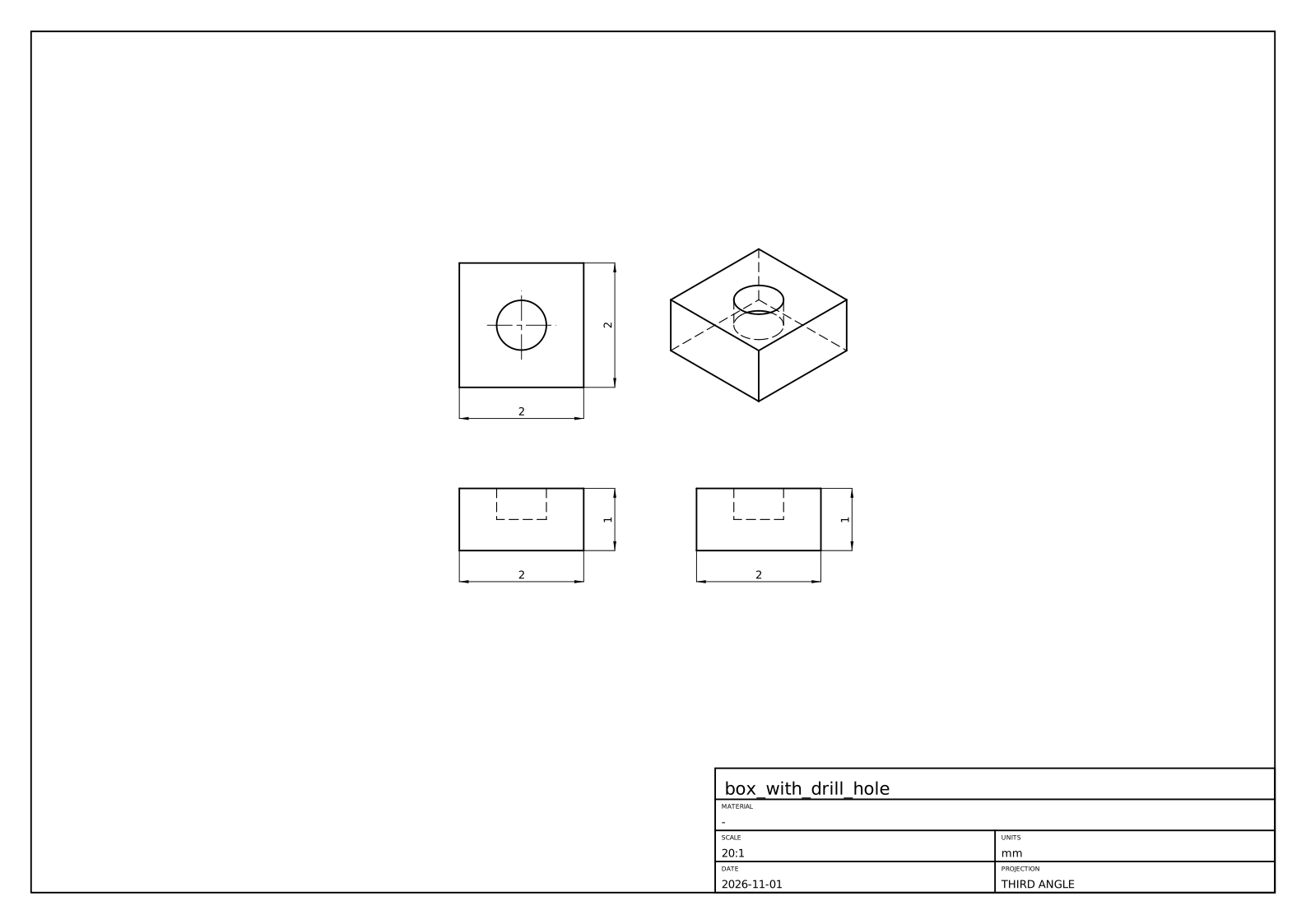
The crate is ops/geop-ops-drawing. Views come from ops/geop-ops-drawing/src/view.rs: “the views are the usual ones of a z-up modeller”. Let us look at how such lines are found.
Hidden-line removal in three steps
What should a view draw? Edges where faces meet at an angle (tangent edges only if asked), and the silhouettes of curved faces. Along such a curve, what is in front of it changes only where its projection meets the projection of another curve, passing behind an edge or a silhouette, or where it turns back on itself. That one observation gives the algorithm (project_view in ops/geop-ops-drawing/src/hidden_lines.rs):
- Project every curve, exactly. Orthographic projection is linear, so a NURBS curve projects to a NURBS curve with the same knots and weights (
ViewFrame::project_curve). - Cut each one wherever its projection crosses or runs along another’s (
curve_curve_overlaps_and_crossings), and wherever it is stationary along the paper’s axes (NurbCurve::stationary_parameters), which holds every point where it turns back. - One point decides a piece. Between cuts, nothing in front of it can change, so a ray from one point towards the eye gives the answer for the whole piece. If it crosses a face first, the piece is hidden.
This is sound, not a heuristic: step 2 removes every place where visibility could change. Look at what step 3 is doing in the context of “Do not decide from samples”: it takes one sample because the structure has proved the answer is constant along the piece. (That is the same shape of argument as Lecture 19 with faces and rays, and as a classification after remesh, Lecture 22.)
Three subtleties, all in seen:
- A crossing at the ray’s own start is no crossing: the point lies on the faces it bounds.
- A crossing on a face’s trim boundary means an edge is in front. The piece runs along that edge on the paper. So it is classified hidden, and a later pass (
drop_drawn) drops it along with every piece lying on one already drawn. A hidden line under a visible one is never drawn, nor any line twice. - A ray running in a face’s surface is seen edge-on, and “an edge-on face hides nothing”:
curve_surface_overlapscatches it first.
Silhouettes
A cylinder seen from the side has two straight lines that are no edge. They are where the surface turns away from the eye. For a view along $d$, a point of the surface is on the silhouette when the normal is square to $d$:
$$g(u,v)=\bigl(S_u(u,v)\times S_v(u,v)\bigr)\cdot d=0.$$
This is a curve in $(u,v)$, and the kernel’s method (ops/geop-ops-drawing/src/silhouette.rs) is the one you know for an intersection (Lecture 16): a seed, then predictor-corrector steps along the tangent $(-g_v,g_u)$, then Newton back onto $g=0$.
Where do seeds come from? $g$’s sign is sampled along a grid of iso lines, with bisection between opposite signs. Is this a sample deciding an answer, against our rule? The comment is careful: “Sampling only decides where to look: what is traced is the exact zero set”. What could it miss, though? A closed loop crossing no grid line lies within one cell, and encloses a critical point of $g$, so each cell where $g$ could vanish is halved into boxes, those that could hold a critical point halved again, and a line through each is sampled too (loop_seats). The grid’s interior lines sit at irrational fractions of the domain, a free choice so they do not run along the symmetric iso lines silhouettes so often are.
Then each piece is trimmed against the face and fitted as a 3-D curve through exact silhouette points, widened to enclose what lies between (NurbCurve3D::fit_enclosing). The visibility test needs a point exactly on it, so it asks Silhouette::exact_point, since a ray grazing a face at its silhouette tells the truth only from the exact point.
A case: the duck’s ankle
A recent commit to this code (c0c70bb4) is a compact lesson in “Name the entities before you name the cause”, from AGENTS.md. Here is what its message records. The duck assembly, updated, did not draw from the right. A vague explanation is easy to imagine: a numerically awkward view. What it named instead: face 37 of the left ankle, the lower quarter cylinder of its D-shaped profile, extruded 15 along $x$; degree 1 along $x$, a rational quadratic round the arc. In the ankle’s frame, the right view looks along $(-1,-8.1\times10^{-15},3.9\times10^{-14})$: 4e-14 off the cylinder’s axis.
So $g$ was a rounding off zero all over the face. Is a silhouette there? Asked to the last bit, the check swept_along said this face is not swept along the view, and the tracer started. Its corrector returned the seed on the start edge at $v=[-50.8,105.5]$, in a domain of $[0,1]$: honest for a $g$ that noisy, but reaching past the domain, and the march then evaluated the arc there, where its weight could be zero.
Two fixes, each of which alone draws the duck. First, the question is asked at the right resolution. A drawing’s resolution is the sheet’s (COARSE_SUBDIVISION), and swept_along now decides to it: every control point of a row, of one weight, within it on the paper of the row’s first. The face then lies within it of the curve its first points span, which its edges draw, and so do its silhouettes. A generator seen 4e-14 off its length projects to a point. Second, the corrector cuts its answer to the domain: the silhouette sought is on the patch, and an interval argument is no licence to evaluate past it. The reproducer is quarter_cylinder_seen_a_hair_off_its_axis, which rebuilds face 37 from its enclosures.
Is the coarse decision an epsilon? It comes close to the line, so here is the reasoning as this book reads it. It does not decide whether a value of the geometry is zero; it decides whether a drawing, whose output is ink on paper, can see the difference, and the fallback when it says no is the edges, which draw the same ink. Compare is_point and the “sheet’s resolution” handoffs in seen. What must not depend on such a threshold is a claim about the geometry itself.
Assemblies, sections, and the sheet
An assembly places the same part a hundred times, and ops/geop-ops-drawing/src/scene.rs is built round that fact.
- Each part on its own: a part’s lines and which of them its own faces hide, from a direction turned into its own frame. Placed parts of one component turned alike share this work.
- The parts together (
Scene::together): each line a part shows is cut where it crosses a line another part shows, each piece decided by a ray against that part’s faces. - Copies behind copies (
Scene::mark_copies_behind): a copy exactly behind another adds no line, so a row of screws seen end on is drawn as one.
A stated limit: “A line is not cut where it enters another part, only where it passes behind its outline: parts that pierce each other are a known limit.”
A section view takes what lies on one side of a plane away, by the kernel’s own boolean: subtract a box standing on the plane from every solid (section_part in ops/geop-ops-drawing/src/section.rs); cut_faces finds what to hatch. No section code runs on its own: a section is a boolean plus the views above.
Then ops/geop-ops-drawing/src/drawing.rs composes: views laid out in third- or first-angle projection, centre marks on circles, overall sizes dimensioned, a border, a title block, and a parts list with balloons if asked for. An Annotation (a Distance, a Radius …) refers to what it measures by the entities’ names and the view’s, and its value is measured anew at each rebuild. “A drawing changes nothing, it only annotates.” It follows the part through every edit because it names things rather than storing positions.
Finally lib/geop-lib-sheet holds plain strokes and labels on layers, written by to_svg or to_dxf. Curves become lines, arcs and circles where they are those (NurbCurve3D::as_line, NurbCurve3D::as_arc), else polylines through points. This is one of the places “Where a user needs the exact line or arc back, as a sketch projecting an edge does, it is reconstructed locally where it is used” from AGENTS.md: the kernel holds a NURBS, and the DXF reader gets a true ARC.
The flat pattern’s DXF of Lecture 33 goes out the same way.
Here is a second real sheet, of rounded_box. Every outline in it is a silhouette: the fillets meet the flat faces tangentially, so the tangent edges are not drawn, and in the isometric view you can see the short silhouette arcs of the ball patches at the corners.
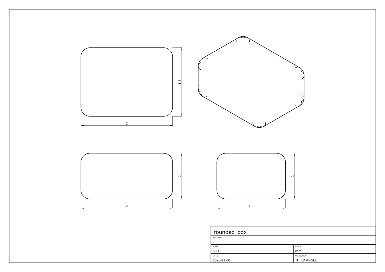
Meshes: the one place that samples
A screen and a 3-D printer want triangles. core/geop-core-rasterize turns a model into sampled geometry: a point per vertex, a polyline per edge, triangles per face, each tagged with the entity it came from, for drawing, picking, STL and debugging.
“Do not decide from samples” names this crate as its exception: “what it draws is a polygon, so sampling is what it is for”. So it is in plain f64, and its quality is a parameter that decides nothing but appearance. Being allowed to sample does not make it easy, though. The problems are combinatorial, not numeric.
The method (triangulate_face, core/geop-core-rasterize/src/grid.rs):
- Every edge is sampled once (
sample_curve), curvature-sized, and a face’s boundaries are placed in its$(u,v)$from those samples, so two faces share exactly the same boundary points. - Pick a uniform
$(u,v)$grid: start from some$n$and double until every cell’s flat approximation is within a curvature tolerance. A flat patch stays coarse, a curved one gets what it needs. - Split the outer boundary and each hole into convex parts, clip each to grid cells (
clip_to_rect), subtract the holes’ parts in each cell (subtract_convex), and ear-clip what is left (ear_clip).
The module comment records three earlier versions that were wrong, a history worth reading: a slit from outer loop to hole that a cell boundary could cross; the same slit done per cell, with a visibility heuristic that could choose a wrong bridge; and clipping a concave outer boundary directly, which returned two pieces joined by a zero-width bridge, so that “a face whose trim went around a hole was drawn across it”. The version that stuck has no bridge to get wrong. A convex region is the intersection of its edges’ half planes, so its complement is the union of their outsides: peel off each outside part in turn.
Two traps
A mesh that ate the machine. AGENTS.md opens its rule “Cap every run’s memory and time” with this. A revolve that “crashed the boolean” was in fact the rasterizer: clipping a concave hole of many corners split it into exponentially many pieces, since subtract_convex kept degenerate leftovers. A concave hole is taken out as many triangles, one after another, and cutting every piece along every triangle’s sides whether it overlaps or not multiplies the pieces with each triangle. The fix is one test: if the leftover inside the hole is empty, the hole does not overlap the subject, and the subject is returned whole. Only interrupting a capped run under gdb showed where it was. The failure surfaced far from its cause, and looking only at the boolean would have found nothing.
A volume that weighed slivers. A closed mesh’s volume is $\sum_T\tfrac16\,a\cdot(b\times c)$, a sum of signed tetrahedra from the origin, by the divergence theorem. Each face was once sampled alone, so two faces met along a curved edge in two polygons a sliver apart: the mesh was not closed. The sum is exact only for a closed figure. Taken from the origin, those slivers were weighted by their distance from it: in a plate at $(10000,-5000,2000)$, AGENTS.md reports 5.5 of error for a bore of 142.
Two fixes, at two levels. enclosed_volume (core/geop-core-rasterize/src/stl.rs) takes its apex at a corner of the mesh, so “what is not closed weighs by its size”. And the mesh itself is now closed: core/geop-core-rasterize/src/mesh.rs makes it conforming, within a face (Mesh::conform) and across an edge (zip), every point any face put on an edge being put on it in every face that edge bounds, bit for bit. “An STL of a solid is a closed mesh.” Note that the mesh’s closure is combinatorial, enforced by construction, not by chance agreement of floats.
Note where exact volume comes from: not this mesh at all. Mass properties integrate the NURBS directly, by Green’s theorem, in core/geop-core-topology/src/mass.rs (Lecture 41). A mesh is for looking at.
Recap
- STEP is a graph of entities mapping nearly one to one onto a B-rep, without required pcurves, with periodic surfaces and closed edges a Geop patch cannot have. Import makes exact NURBS, cuts wrapping faces, and fits pcurves.
- A file’s disagreement becomes enclosure width: union for a vertex, widening for an edge. Past
1e-4, it heals from the surfaces, or refuses by name; what it healed is reported. - Export writes B-splines exactly, midpoints of intervals. A corpus of real files tests the importer; no pass rate is claimed here.
- Hidden lines: project exactly, cut at crossings and turning points, decide each piece with one ray. A silhouette is the zero set of
$(S_u\times S_v)\cdot d$, traced like an intersection. - Decide at the output’s resolution where the output cannot see the difference:
swept_alongto the sheet’s. - The rasterizer may sample since a polygon is what it draws. Its hard problems are combinatorial: runaway piece counts, and a mesh that must close.
Exercises
1. Verify Euler’s formula for the rounded_box STEP counts given above. Then predict $F,E,V$ for a box with one fillet on one edge, and for the same box with a through hole. (For a solid with one hole through it, $V-E+F=2-2g$ with $g$ the genus: but also note Geop requires a face with a hole to have two loops, so the formula needs the number of loops $L$.)
Solution
$24-48+26=2$. One fillet on one edge of a box: the fillet adds one face, and splits the edge into two, with the two end vertices each becoming two: $F=7,E=15,V=10$, and $10-15+7=2$. A through hole: the general form is $V-E+F-(L-F)=2(1-g)$, where $L$ is the number of loops. For example, a plain box with a square through hole has $V=16,E=24,F=10,L=12,g=1$: $16-24+10-2=0$.
2. A file has a vertex whose point is $(1,0,0)$, an edge end at $(1+2\times10^{-7},0,0)$, and a foot on a surface at $(1-10^{-7},0,0)$. What enclosure does the importer build for the first coordinate, and what is its width? Is it accepted? How would your answer change if the edge end were at $1+3\times10^{-4}$?
Solution
The union: $[1-10^{-7},1+2\times10^{-7}]$, widened by rounding, of width $3\times10^{-7}$. That is far under ACCURACY, $10^{-4}$, so it is kept. At $1+3\times10^{-4}$ the places lie further apart than the kernel can carry as one point, so heal rebuilds the vertex where its faces’ surfaces meet, if they meet within the file’s uncertainty near it, and reports how far it moved in a Healing. If they do not, it either leaves out the smallest faces and rebuilds them from their edges, or refuses by name.
3. In the hidden-line demo, choose “one box” and turn it to any general view. Count visible and hidden edges. Show that a convex polyhedron seen from a general direction shows an edge if and only if at least one adjacent face is front-facing. Why does the algorithm in the demo not need that rule, and what would it miss if it used only that?
Solution
A box shows 9 and hides 3 from a general corner view. For a convex solid a point on a front-facing face has nothing in front of it: the solid lies entirely behind the face’s plane. An edge between two back-facing faces lies behind them. The rule is special to convex solids and to a solid hiding itself alone: with two solids, or with a non-convex part, a front-facing face can still be behind something. The ray from each piece asks about everything in front, so it needs no such rule, and it is correct for the general case once cuts are in the right places.
4. Why must a curve be cut where its projection is stationary along the paper’s axes? Give an example of a curve that is seen wrongly if you cut only at crossings with other curves.
Hint
The module comment says it: a turn-back is where a curve runs along the line of sight. A planar arc seen nearly edge-on projects to a line traversed twice. Without a cut at the turn, one piece covers both directions, one visible and one hidden, with no crossing between them. The stationary points also leave every piece monotone along both axes, which the module uses for other purposes.
5. Find $g(u,v)$ for a cylinder of radius $R$ about the $z$ axis, with $S(u,v)=(R\cos u,R\sin u,v)$, viewed along $d=(d_x,d_y,d_z)$. Where is the silhouette? What happens as $d\to(0,0,1)$, and how does this relate to the duck’s ankle?
Solution
$S_u\times S_v=(R\cos u,R\sin u,0)$, so $g=R(d_x\cos u+d_y\sin u)$, zero at $u=\operatorname{atan2}(d_y,d_x)\pm\pi/2$: two generators. As $d$ approaches the axis, $(d_x,d_y)\to0$, and $g$ tends to zero everywhere: every point is a silhouette, and each generator projects to a point. In the limit the whole lateral face has no silhouette to draw, only its end circles. When $(d_x,d_y)\approx4\times10^{-14}$, $g$ is rounding, as on the ankle. That is why swept_along has to recognize the case rather than trace $g$.
6. Suppose a mesh is not closed: there is a gap along a curved edge of length $\ell$ and width $\epsilon$. Estimate the volume error of the tetrahedra sum from an apex at distance $D$. Now take the numbers in the text, and check that $D\approx10^4$ and a sliver of area $\sim10^{-3}$ give the right order of error.
Solution
The sum over a closed mesh is independent of its apex. A mesh with a hole of (vector) area $A$ adds an apex-dependent term $\tfrac13D\,A$ in magnitude: a missing face’s own tetrahedron. With $A=\ell\epsilon$, $D\sim1.1\times10^4$, the error is about $3700\,\ell\epsilon$, and 5.5 corresponds to $\ell\epsilon\sim1.5\times10^{-3}$, plausibly a rim’s length of 40 by a sliver of $4\times10^{-5}$. These sliver numbers are an estimate, not measured. Placing the apex on the mesh makes $D$ the part’s own size, reducing the error to $\sim80/1.1\times10^{4}$ of that.
Lecture 36: Mates and poses
After this lecture you can
- represent a rigid motion by a quaternion and a position, and say what happens when the quaternion is off unit;
- explain why a solver must step a pose by a twist through the exponential map, not by adding to a global coordinate;
- write a mate or a joint as residuals, and count its rows and the freedom it leaves;
- explain why a joint’s angle row is
$2\tan\frac{\varphi-\theta}{2}$, not a sine; - say what a mate means when the user picked a piece of a wall, and why a reference direction must not be left to noise.
A part is rarely alone. A hinge has two leaves and a pin; a robot has hundreds of parts. An assembly in Geop is a part in which other parts are placed, each another file’s program, and mated: a statement about how a placed part sits relative to something else. “This shaft is concentric with that hole.” “This link turns about that axis.”
The sketch solver of Lecture 23 moved numbers. Here the unknowns are positions and orientations of rigid bodies, and the same System will solve them (Lecture 37). What is new is that a rotation is not a number: it does not live in a vector space. This lecture is about how to make a Newton-type solver work on such a thing, and then how to state a mate.
four_bar example, four files placed and mated, meshed by the real kernel. In the editor, drag a link and the others follow, solved live.Where a part is
A placed part’s location is a value of the program’s state: not an argument of the step, and not something the step computes. In a saved program it looks like this:
"state": { "pin.pose": { "position": [1.0, 1.0, 0.5], "rotation": [1.0, 0.0, 0.0, 0.0] } }
The step AddPart (ops/geop-ops-assembly/src/add_part.rs) places the part where that state says and adds its mates. It solves nothing. A solve outside the part moves the state until the constraints hold (Lecture 37). So a mate in a later step can move a part an earlier step placed, for every step.
That pose is Pose in core/geop-core-math/src/primitives/pose.rs: a point $p$ of the part is at $Rp+\text{position}$, with $R$ the rotation of a quaternion.
Rotations by quaternions
A rotation by angle $\theta$ about a unit axis $n$ is the unit quaternion
$$q=\Bigl(\cos\tfrac\theta2,\ \sin\tfrac\theta2\,n\Bigr),$$
and it turns a vector $v$ by the product $qv\bar q$, with $v$ treated as the quaternion $(0,v)$. Composition of rotations is multiplication of quaternions. For example a quarter turn about $z$, $q=(\tfrac{\sqrt2}{2},0,0,\tfrac{\sqrt2}{2})$, sends $(1,0,0)$ to $(0,1,0)$. Note that $q$ and $-q$ give the same rotation: the half angle means a full turn of the body goes half way round the quaternions.
Why quaternions, and not matrices or Euler angles? A rotation matrix has nine numbers and six conditions, which rounding violates. Euler angles have three numbers but go singular at gimbal lock; in Geop, angles are for showing a pose to people only (Pose::euler_degrees, Pose::from_euler). A quaternion has four numbers and one condition, and if the condition is off by a hair, it can be handled.
The kernel’s choice is that a quaternion need not be unit to stand for a rotation: the rotation it makes divides by its norm squared (see Pose::apply). That is a deliberate decision and it pays off in two places.
A value read from a file is kept as read. Pose’s reader used to normalize the quaternion it read. Normalizing a sharp quaternion gives an interval. A file holds its midpoint, which reads back as another interval and is written as another midpoint. A program with a placed part’s pose in its state was never the same program once saved and loaded, and the press example failed its round trip (AGENTS.md). So the reader keeps the pose exactly as read and refuses only what stands for nothing, the zero quaternion. Reading what was written must give back what was read.
An enclosure must hold a rigid motion. Where the proof needs a unit quaternion, it normalizes honestly, in intervals, as Lecture 24 told: retract_over.
The coordinates a solver moves in
Newton’s method needs an update $x\leftarrow x+\delta$. A pose has no plus. What should a step of a pose be?
The tempting answer, and the kernel’s former one, is a global chart: a body’s turn is described by a 3-vector $w$ through the quaternion $(1,w/2)$, normalized. It is smooth, has three numbers, and is the identity at zero. It looks perfect. Take a turn about $z$: $(1,w/2)$ normalized has half angle $\arctan(w/2)$, so the angle it stands for is
$$\theta(w)=2\arctan\frac w2,\qquad\frac{d\theta}{dw}=\frac{1}{1+w^2/4}.$$
Look at that derivative. A half turn is reached only as $\lvert w\rvert\to\infty$. To stand at $170°$, $w=2\tan85°\approx22.9$. At $179.5°$, $w\approx458$, where one unit of $w$ turns the body by only $2\times10^{-5}$ radians. The Jacobian’s column has shrunk by that factor, and the solver’s damping, which keeps a value near where it was, now weighs more than the motion.
From AGENTS.md: a link of a dragged arm that had to turn nearly half way round ran its variables off to hundreds, each step turning it less, until the solver ran out of steps. Nothing was wrong with the mates. The coordinate system simply could not reach the answer at a finite, well-conditioned value.
2e-6 off, with w at 458. Blue steps a twist from where the body is: 11 and 12 steps. Slide the target and the damping.Twists and the exponential map
The fix is to stop having a global coordinate at all. Every step of the solve is taken from where the body is:
$$x\oplus\delta=x\circ\exp(\delta).$$
Here $\delta=(\omega,v)$ is a twist, six numbers in the body’s own frame: turning at $\omega$ while moving at $v$, for unit time. It is a tangent vector at $x$, and $\exp$ takes it to the rigid motion it generates. Since $\delta$ is measured from the current pose, every step’s coordinates are close to zero, where the map is perfectly conditioned. No turn is ever far from the variables’ origin. A half turn is just two quarter turns.
A solver usually calls this operation a retraction, which is the name in the kernel’s trait: Variable::retract. The trait in core/geop-core-math/src/solvers/system/mod.rs is how the generic solver sees any value it moves: dimension, retract (where a step takes it, sharp, a seed), retract_over (every value a box of steps takes it to, an enclosure), differential, stay, same, carried. A number is one instance, with retract being addition. A pose is another, with dimension 6.
The formula. For $\omega$ with $\phi=\lvert\omega\rvert/2$, Pose::exp computes the unit dual quaternion $\exp(\hat\xi/2)$ of $\hat\xi=\omega+\varepsilon v$, which multiplied out gives
$$\text{rotation}=(\cos\phi,\ s\,\omega),\qquad\text{position}=2s\cos\phi\,v+(s^2+2c\cos\phi)(\omega\cdot v)\,\omega+2s^2\,\omega\times v,$$
with
$$s=\frac{\sin\phi}{2\phi},\qquad c=\frac{\cos\phi-\sin\phi/\phi}{8\phi^2}.$$
It is a screw motion along the axis of $\omega$: it turns by $\lvert\omega\rvert$ radians. To first order, it is $(1,\omega/2)+\varepsilon(0,v/2)$. Near $\phi=0$ the closed forms are $0/0$, so Pose::exp sums them as series in $\phi^2$, polynomials and smooth through zero. Each series alternates, and for $\phi^2<1$ its terms shrink, so each sum is within its first omitted term, which is added as an honest enclosure. So the map is an enclosure for a twist that is a box around zero too, and so are its derivatives. Dual numbers can differentiate straight through it, as a solver does to linearize a pose (Pose::exp_with_derivatives).
A worked example. Let $\omega=(0,0,\pi/2)$, $v=(1,0,0)$: a quarter turn about $z$, moving along the body’s own $x$ throughout. Then $\phi=\pi/4$, $s=\sin\phi/(2\phi)=0.4502$, and $\omega\cdot v=0$:
$$\text{position}=2s\cos\phi\,(1,0,0)+2s^2\,(0,\tfrac\pi2,0)=(0.6366,\ 0.6366,\ 0).$$
Indeed: a point moving at speed one while turning through $\theta=\pi/2$ traces a quarter circle of radius $1/\theta$, from the origin to $(\sin\theta/\theta,\ (1-\cos\theta)/\theta)=(0.6366,0.6366)$. The demo’s test, book/scripts/demo_tests/pose-exp.test.mjs, checks this formula against numerically integrating the motion.
The differential. For Lecture 24’s proof we need the Jacobian of a term by the step at every point of a box. That is the term’s Jacobian by the steps at $x$, what Equations gives, times the differential of the retraction: for a pose, the right Jacobian of the exponential map (Variable::differential, by Pose::exp_differential). At a step of exact zeros, it returns None: the identity, exactly, with no rounding introduced.
Staying put. What holds a part where it was when nothing else decides? Variable::stay gives residuals: its position’s difference from at, and its rotation’s as the unit quaternions’ difference, using the nearer of $\pm$, times scale, so that a turn counts as the distance it moves a point that far from its axis. Everything in a system of residuals is again a length.
Mates as residuals
A Mate holds a MateKind between MateEntitys (ops/geop-ops-assembly/src/mates.rs), of four sorts:
- Constraints (
Kind):Coincident,Concentric,Parallel,Perpendicular,Distance,Angle,Tangent,Path. Each takes a point, a line or a plane of each entity, where its part puts it. - Joints (
JointKind,Joint): how the second frame may move on the first. Revolute, slider, cylindrical, planar, pin in slot, ball, universal, fastened. - Couplings (
CouplingKind): a coordinate of one joint tied to one of another by a factor and an offset: gear, belt, rack and pinion, screw, linear. They are presets of one linear relation. - Fixed (
Anchor::Fixed): of one entity, or, in anadd_partstep, of none, meaning the part that step places. The part never moves in a solve.
Each is residuals. Take residuals in ops/geop-ops-assembly/src/residuals.rs, with everything computed in dual numbers so every residual carries its derivatives:
| Mate | Entities | Rows | Residual |
|---|---|---|---|
| Coincident | point, point | 3 | $p-q$ |
| Coincident | point, plane | 1 | $n\cdot(p-q)$ |
| Coincident | point, line | 2 | $p-q$ along two directions across the line |
| Coincident | line, line | 4 | parallel (2), one point off the other line (2) |
| Coincident | plane, plane | 3 | parallel (2), one on the other (1) |
Note how “parallel” and “off a line” are always two rows across the direction. A vector cross product has three components and rank two, which would give a redundant row at every solution, right at the point the Krawczyk test wants independence. Choosing rows in a basis across the direction avoids having to detect it. Picking what you ask for is cheaper than a rank decision.
One table of joints
Joint::frees is one table: how each joint lets the second frame turn, and the motions it frees as coordinates. Every one is held by one residual function, joint_residuals in ops/geop-ops-assembly/src/joints.rs. The second frame’s origin must be at the first’s, moved along its axes by the joint’s slides. Its axes must be turned about the first’s $z$ by its angle, or kept square to it for a universal joint’s cross, or free for a ball.
| Joint | Coordinates | Rows | Freedom |
|---|---|---|---|
Fastened | none | 3 + 2 + 1 | 0 |
Revolute | angle | 3 + 2 + 1 | 1 |
Slider | slide | 3 + 2 + 1 | 1 |
Cylindrical | angle, slide | 3 + 2 + 1 | 2 |
PinSlot | angle, slide $x$ | 3 + 2 + 1 | 2 |
Planar | angle, slide $x$, slide $y$ | 3 + 2 + 1 | 3 |
Universal | none as a coordinate | 3 + 1 | 2 |
Ball | none as a coordinate | 3 | 3 |
Count a revolute joint between a fixed body and a free one. The variables are the body’s pose (6) and the coordinate $\theta$ (1): seven. The rows are 3 for the origin, 2 for the axes parallel, and 1 for the turn: six. $7-6=1$. That is what a hinge should have.
The coordinate is a variable. $\theta$ is a value of the state, named after the mate (joint_parameter: add_part(arm2,m1).angle), that can be set, held, or limited. Its Mobility is Follows: move it as the constraints have it, and hold it nowhere. It follows its parts, since held as well, it would pull against them.
A ball’s and a cross’s turn is no coordinate at all, because angles of them go singular. Do not make a value of something with no good global coordinate: that was the lesson of the demo.
The angle row, and a free choice that matters
How should “$b$’s reference is turned from $a$’s by $\theta$” be written? Let $u$ be $a$’s reference turned by $\theta$, let $t$ be its direction a quarter turn on, and let $r_b$ be $b$’s reference. The obvious candidates are bad:
$r_b-u$, the difference of two unit vectors. The component along$u$vanishes to second order. At a solution reached to tolerance, this row has a slope as small as that tolerance and still counts as a constraint, pinning the joint. This is the “redundant row looks independent” of Lecture 24, self-inflicted.$\sin(\varphi-\theta)=r_b\cdot t$, with$\varphi$the true angle. One row of slope one, except that a sine is zero half a turn away as well. The solve can land on the wrong branch.
The kernel’s row is
$$2\tan\frac{\varphi-\theta}{2}=\frac{2\,r_b\cdot t}{1+r_b\cdot u}.$$
Zero only at $\varphi=\theta$, one row, slope one there. (Check: $r_b\cdot t=\sin(\varphi-\theta)$ and $r_b\cdot u=\cos(\varphi-\theta)$, and $\tan(x/2)=\sin x/(1+\cos x)$.) Half a turn away the denominator goes to zero and the row fails, honestly: infeasible, a step turned down. Then it is multiplied by the scale $\ell$, to be a length.
What a pick means
Here is something a solver’s author would never guess. A cam swept along a sketched circle is four faces, a quarter each, and a follower held tangent to the one picked ran to its end and stopped: the solve met the foot point’s limit a quarter turn on. Nothing was wrong with the solve. What the user picked was the wall, and the face was only a piece of it (AGENTS.md, A face is a piece of a wall).
A Tangent mate keeps a circle (a roller’s rim, a pin’s) its radius off a face. A Path mate keeps a point on a curve. Where on it is the foot point, whose parameters are values of the state (foot_parameter: add_part(follower,m2).u), solved with the poses. Its residuals are the follower’s point less the foot point.
Now mate_entity::wall in ops/geop-ops-model/src/mate_entity.rs takes a face and joins it with every face it runs on into across an edge, tangent to it, into one surface (NurbSurface3D::joined). The faces are taken in the order of their ids, since a hash map’s order is no order. And mate_entity::run does the same for an edge and the edges it carries on into. A parameter along which the joined wall closes on itself wraps round instead of ending; one along which it does not is kept within its domain by limits. So a follower now rolls round every face of a cam.
Where a pick names a piece of something the geometry continues, ask whether the operation means the piece or the whole.
A reference direction is not left to noise
A joint measures its turns from a direction square to its axis, chosen from the world’s axes as the one the axis runs least along. An axis along $z$ is a hair off it in $x$ and in $y$ alike. So which of the two is least was decided by noise, differently for the two ends of a joint: a quarter turn or none.
Vector3::across in core/geop-core-math/src/vector/linalg.rs takes the first axis that no other component is definitely less than. For an interval-valued axis this is stable: if $x$ and $y$ components could be equal, neither is definitely less, so the choice falls on the first one, at both ends. It is the interval version of “use a tie-breaker that does not depend on noise”. And a frame put on a face or an edge, frame_along in ops/geop-ops-model/src/geometry.rs, gives the same direction the joint would have chosen. So frames and the entities they are on are at a turn of zero alike, and a joint clicked on a hole begins at angle zero.
In the kernel. Poses: core/geop-core-math/src/primitives/pose.rs (Pose::exp, Pose::exp_differential, impl Variable for Pose). Mates: ops/geop-ops-assembly/src/mates.rs, ops/geop-ops-assembly/src/joints.rs, ops/geop-ops-assembly/src/residuals.rs. What a mate’s steps declare: ops/geop-ops-assembly/src/mechanism.rs (constraints through define_constraints, unknowns through declare_unknowns). Elements: MateEntity in ops/geop-ops-model/src/mate_entity.rs. Limits are constraints of their own, Bound::AtMost.
Not implemented: the solver knows nothing of collision. Parts pass through each other unless mates forbid it. MotionPanel plays a motion study and can ask the interference inspector about every frame (Lecture 37), but no contact is solved other than a Tangent or Path mate. Interference on a whole assembly can be asked of some parts only (Scope in ops/geop-ops-inspect/src/scope.rs), and asks could_touch of each pair rather than the least distance; stopped part way, the answer says how far it got (Stopped), since what was not looked at is unknown.
Recap
- A pose is a quaternion and a position. The quaternion need not be unit; the reader keeps what it read; an enclosure normalizes honestly.
- A global coordinate of a turn reaches half a turn only at infinity. Steps are twists from where the body is, through
Pose::exp, and no turn is ever far from the origin of the variables. - A mate is residuals, each a length. Rows are chosen in a basis across a direction, so that redundancy does not arise by construction.
Joint::freesis one table,joint_residualsone function. The angle row$2\tan\frac{\varphi-\theta}{2}$is the one with slope one and a single zero.- A pick may name a piece of a wall or a run: ask what the geometry continues. A direction chosen from data needs a tie-break the noise cannot flip.
Exercises
1. Compute $qv\bar q$ for $q=(\cos\frac\theta2,0,0,\sin\frac\theta2)$ and $v=(1,0,0)$, and confirm the result $(\cos\theta,\sin\theta,0)$. Now scale $q$ by 2 and apply $qv\bar q$ without dividing. What comes out, and what must Pose::apply do?
Hint
Expanding gives $(\cos^2\frac\theta2-\sin^2\frac\theta2)\,e_x+2\sin\frac\theta2\cos\frac\theta2\,e_y$. Scaled by 2, the result is 4 times longer: $\lvert q\rvert^2$. So applying a non-unit quaternion divides by its norm squared.
2. In the model problem, a pull with damping $\mu$ and slope $\kappa=d\theta/dw$ near the target gives the step $\delta w=-\kappa r/(\kappa^2+\mu^2)$, with $r$ the angle error. Show that the angle error then shrinks per step by the factor $\mu^2/(\kappa^2+\mu^2)$. Evaluate it at $179.5°$ with $\mu=10^{-4}$. How many steps to gain a factor of $10^6$?
Solution
$\delta\theta=\kappa\,\delta w=-\frac{\kappa^2}{\kappa^2+\mu^2}r$, so the new error is $\frac{\mu^2}{\kappa^2+\mu^2}r$. At $179.5°$, $w=458.4$, $\kappa=1/(1+w^2/4)=1.9\times10^{-5}$, $\kappa^2=3.6\times10^{-10}$, $\mu^2=10^{-8}$. The factor is $0.965$. Then $\ln10^6/\ln(1/0.965)\approx390$ steps, past the demo’s cap of 200 as it shows. With a twist, $\kappa=1$ always, and the factor is $10^{-8}$ per step.
3. Evaluate Pose::exp’s position formula for $\omega=(0,0,\pi)$, $v=(0,0,1)$, and interpret the motion. What about $\omega=(0,0,0)$, $v=(a,b,c)$? Why can’t the code use the closed form for $s$ and $c$ there?
Solution
$\phi=\pi/2$, $s=1/\pi$, $\cos\phi=0$, $c=(0-(1/(\pi/2)))/(8\pi^2/4)=-(2/\pi)/(2\pi^2)=-1/\pi^3$. Then $2s\cos\phi\,v=0$, $\omega\cdot v=\pi$, $(s^2+0)\,\pi\,\omega=(1/\pi^2)\pi(0,0,\pi)=(0,0,1)$, and $\omega\times v=0$. Position $(0,0,1)$: half a turn while advancing by one, a screw. For $\omega=0$: the formula gives $v$, a pure translation, using the limits $s=\frac12$, $\cos\phi=1$. The closed form has $\phi$ in the denominator, $0/0$, hence the series.
4. For a Cylindrical joint between a fixed body and a free one, count the variables and rows. Do the same for a Ball. What if two Revolute joints on parallel axes join the same two bodies?
Solution
Cylindrical: 6 + 2 coordinates = 8 variables, 3 + 2 + 1 = 6 rows, freedom 2. Ball: 6 variables, 3 rows, freedom 3. Two revolutes, coaxial: 6 + 2 = 8 variables, 12 rows, rank 7: freedom 1, 5 rows redundant. If their axes are parallel and distinct: the rows cannot all vanish, since no pose has its axis on both. That is a conflict of the geometry, not of the arithmetic, which conflicting reports.
5. Verify that $2\tan\frac{x}{2}=\frac{2\sin x}{1+\cos x}$ has slope one at $x=0$ and no other zero in $(-\pi,\pi)$. Show that the component of $r_b-u$ along $u$ has zero slope in $x$ at $x=0$, and explain with Lecture 24 what this would do to a rank decision.
Solution
With $x=\varphi-\theta$, $r_b\cdot u=\cos x$, so the component of $r_b-u$ along $u$ is $\cos x-1\approx-x^2/2$: slope $-x$. At a solution to tolerance, $x\approx10^{-9}$ gives a pivot of $10^{-9}$, small but maybe definitely not zero, so it counts as an independent row, and pins $\theta$ to $\varphi$ where there is no such constraint of its own beyond the single turn row. That is exactly how a redundant row looks independent at a point.
6. Why is a wall’s seam, in mate_entity::wall, handled by wrapping a parameter, rather than by keeping the foot point on one face and switching faces when it reaches an edge?
Hint
A solver’s variables must be smooth: switching faces is a discontinuity in $f$ and $J$, where no Newton step is valid and the rank test may disagree on each side. On one joined surface, with a parameter wrapping round, the foot point moves continuously across what were edges. It is also the same trick as Coincident: remove the case from the equations, by construction.
Lecture 37: The assembly solver
After this lecture you can
- describe the loop that solves a program’s state from outside the part, and why no step writes the state;
- compute a mechanism’s freedom from the rank of its rows, and say where counting formulas go wrong;
- explain groups and pendants, why they are the difference between a small system and a cubic one, and how the rank test behind a pendant must be asked;
- tell a limit position from a singular configuration, in a real linkage;
- say what the editor does after every edit, what a conflict report costs, and why a value must be read where its read is checked.
Lecture 36 wrote mates and joints as residuals. Now we solve them, while a user drags a link, in an assembly that may have 2000 parts. The numerics are exactly those of Part VI, since the same System in core/geop-core-math/src/solvers/system/ does the work: least_squares::minimize steps, Krawczyk proofs, rank over a box. What is new is scale and structure. A dense solve is cubic in its variables, and 2000 parts have 12 000 of them. The lecture’s main idea is the observation that makes this tractable: a real assembly is nearly all parts that merely hang off a few that matter.
The loop outside the part
From Lecture 2: a program is a list of steps that builds a part. Where the placed parts are is the program’s state, an input. A step declares what it requires of the state and which values a solve may move, in two targets of the part:
Constraints, residuals to vanish (or, for a limit,Bound::AtMost, to stay at most zero), with their derivatives. A step defines them throughdefine_constraints, andConstraints::ofgathers every step’s. These are inlib/geop-lib-constraints/src/constraint.rs.Unknowns (lib/geop-lib-constraints/src/unknown.rs): a state value, itsMobility, aseedfor where to start it, andunless, a constraint which, if it fails, says to start it from the seed.Unknowns::ofgathers them.
Mobility says what a solve may do with a value:
Mobility | Meaning | Example |
|---|---|---|
Fixed | stays exactly as it is | a part with a fixed mate |
Held | moves as far as the constraints need, and no further: held by DAMPING | a placed part’s pose |
Follows | moves as the constraints have it, held nowhere | a joint’s coordinate |
So the solve happens outside the part. solve in lib/geop-lib-constraints/src/solve.rs runs the part at the state once, reads its constraints, and steps the state. At every state it tries, it does not run the program again. It makes only the constraints it asks again, each by its step’s generator, of the part as built and the state tried (Remade). So the work of a solve step is that of the constraints it asks. No step writes the state, and every front end gets the same solver.
Preferences, which become the system’s preferences as in the sketch’s solve, express what a solve should favour among the states the constraints allow: a drag is Pull::Point, a point of a placed part pulled towards the pointer. Typed-in placement is Pull::Pose, and setting a joint is Pull::Value, which holds that coordinate at its value and lets the parts move to it (Pull in core/geop-core-editor/src/editing/form.rs).
Freedom, by rank
Here is a planar four-bar linkage: a crank, a coupler and a rocker on two ground pivots. Each moving body has a pose (in the plane, $x,y$ and an angle, three numbers). Each pin takes two rows. So 9 variables, 8 rows: $9-8=1$. One way to move. That is the classic Grübler count: 3 per body minus 2 per pin.
Grübler counts rows. The kernel uses their rank, for the reason you met in Lecture 23. Take a parallelogram linkage, whose coupler always stays parallel to the ground, and add a third crank midway, parallel to the other two. It adds one body (3) and two pins (4): 12 variables, 12 rows, and Grübler says 0: it cannot move. And yet it plainly moves, since the third crank follows the motion the first two already determined. The row that the third crank’s closing pin adds is redundant: rank 11, freedom 1. Everywhere, not at one point.
Two kinds of “stuck”
The demo shows the two things that can look like lock-up. They are very different.
A limit position. In the crank-rocker linkage, press “Rocker’s limit”. Crank and coupler now lie on one line, and the rocker has reached the end of its swing. Read the numbers: the rank is still 8, the freedom still 1, regular. The linkage’s one motion has the crank turning and the rocker standing still (the readout’s rate goes to 0). If you drag the crank, it just keeps going. If you drag the rocker past its limit, it stops, at the end of its travel, as the pull’s minimum among where the pins hold. Machinists call this a dead point, since a rocker driving the crank has no leverage there. For the solver nothing special has occurred.
A singular configuration. Press “Flat parallelogram”. All four pivots lie on one line. The rank drops to 7, the freedom to first order is 2, and the smallest pivot is zero. There really are two ways out: staying a parallelogram, or folding into an anti-parallelogram with the coupler crossing. This is what a Krawczyk proof cannot pass: a singular point, like the tangent of Lecture 24. As System::enclose would put it, no true solution is proven there, and Report says so. A step of a drag lands a hair away from it on some branch, and the rank is back.
The constrained minimizer has seen this too: its curvature estimate $B$ can change abruptly across such a configuration, so where a step it proposed is turned down, the step is tried again without it, and it is learned afresh if that does better (core/geop-core-math/src/solvers/least_squares.rs). It is also why no merit function is used: $\Sigma r^2+\rho\lvert c\rvert$ would need $\rho$ above the multipliers, and those grow without bound at a singular configuration, the module’s comment says, two links in line for example.
Scale: a benchmark has to have the shape of the real thing
From AGENTS.md’s Count the work, not the seconds: the 2000-part robot benchmark mated every screw to a fixed plate, so the solver split it into 2000 groups of one screw, and drags were fast. A real robot mates screws to brackets fastened to links that turn: one group of every part. The robot_arm benchmark (ops/geop-ops-assembly/src/testing/robot_arm.rs) has that shape: a fixed base and a chain of links on revolute joints, brackets fastened to the links, screws mated to the brackets, motors, belted pulleys and a gripper. And a drag of only 101 of its parts ran for over fifty minutes without finishing: one dense system of 600 variables.
Groups
The first step in System::structure (core/geop-core-math/src/solvers/system/structure.rs) is the obvious one. Blocks no term ties together are separate systems, found by union-find over which blocks each term reads (grouped). A plate with hundreds of screws is hundreds of systems of one screw. The answer is the same, as what a solve minimizes is a sum over the groups, and a group whose constraints hold and that nothing pulls is not solved at all. A question about the system splits likewise: freedom in lib/geop-lib-constraints/src/solve.rs measures group by group.
That helps the plate. It does not help the arm, in which everything is connected.
Pendants
Think about a screw mated to a bracket. The screw’s constraints read the screw and the bracket, and they decide nothing about the bracket. Whatever the bracket does, the screw can follow, and how it does is the screw’s own business. Such a block is a pendant on the blocks its terms read besides it: it can be solved after them, alone, with them where they ended up, and enclosed after them, over their boxes. After taking the screw off the bracket, the bracket comes off its link the same way. What is left is the core: the links and joints.
A block $b$ hangs off the blocks $S$ its remaining terms read besides it when, where the blocks are:
- Nothing pulls it, and no limit reads it. Either could hold back what it hangs off.
- Its terms hold. It is where they put it, given
$S$. - Its rows have the same rank by its own steps as by all of
$S$’s and its own. They constrain nothing of$S$, to first order. A part mated to a link and to the ground is no pendant, since its rows also hold the link. - It can be carried. Held where it is, it can be moved along by one of
$S$(Variable::carried,$to\circ from^{-1}\circ self$for a pose), which is what a solve starts it from. And every value of$S$that onlyFollowsmust still be read by some other term. Otherwise a joint coordinate only$b$’s joint reads would be held where it was, and$b$turned with the link, where the whole solve held$b$and turned the joint.
The third condition is a rank decision, and it has the same trap as in Lecture 24. From AGENTS.md: the rank test was first asked at the point. Rounding leaves a hair of a row that depends on the others, $10^{-17}$, definitely not zero, and nothing was a pendant off the axes. Asked over a box as wide as the solver’s tolerance, as the enclosure asks it, it could be zero. “Decide a rank over the box” holds for every rank decision, not only the enclosure’s.
The result is layers (Structure::layers). Each Group has blocks and the blocks on which it depends, in an earlier layer. The arm’s drag is then its links and joints, 42 variables, however many parts hang off them (AGENTS.md). The groups of a layer are worked on in lockstep (core/geop-core-math/src/solvers/system/lockstep.rs): one evaluation answers every group waiting, so the evaluations a solve takes do not grow with the number of groups.
What changes in the answer? Only what a block “held where it was” holds back. A pendant moves with what it hangs off, and of its own freedom stays as near where it was as its terms let it. But it no longer holds back what it hangs off: a link carrying a hundred screws is as easy to move as one carrying none. For a user that is simply better.
Counting instead of timing
AGENTS.md tells the rest. A drag in a 2000-part robot went from 0.25 s to minutes, and nothing timed it. The editor builds every step’s form on every change, for the step list; the added part’s form asked the whole assembly how free its part was, a dense null space over every part’s variables. Once per step, that is cubic in the parts. Now:
- A form shown in a list is of the step’s arguments and the program’s state. Questions about what was built, over the whole assembly, are for the one dialog open, once per edit.
- Guards are counts, not times.
geop_ops_assembly::mates_resolvedcounts mates found and measured, andops/geop-ops-assembly/src/scale_tests.rsasserts on it: building 30 screws on a plate resolves 31 mates, and a part moved resolves none, since “only screw7’s constraint reads where it is”.workincore/geop-core-math/src/solvers/mod.rscounts dense linear algebra as$\text{rows}\times\text{columns}^2$for each factorisation, so a test can bound a solve’s cost. A quadratic shows at 80 parts as clearly as at 2000. - An event of a drag changes the state alone (
Changed::State). It sends the parts it moved, and the program once the drag is let go. - A drag’s events are a hair apart, so the structure found in one is reused for the next (
Problem::structure,System::solve_unproven_in) rather than found again. If a pendant cannot follow after all, the check notices.
Lecture 41 returns to all this.
What the editor does
The assembly crate adds to the editor through one trait, Settle in core/geop-core-editor/src/registry.rs, which is what keeps the kernel from knowing about mates. After every edit, Settler::settle in ops/geop-ops-assembly/src/settle.rs does the following.
- If something pulls, pull first: every part not fixed is free to give way. A linkage follows the link dragged.
- Otherwise, if the mates hold, nothing moves at all.
- Otherwise solve for the step’s own part first, the others held: mating a new part moves it, not the part it is mated to. Only if that does not converge is every part not fixed set free.
- Where the constraints still do not hold, ask which conflict.
A Report from a solve carries what holds, the limits stopped at, what moved, the minimizations and an Enclosure for every group, or why none: the constraints that conflict, by name, or what is singular.
Limits (Bound::AtMost) are kept by an active set: solved without the limits first, then every one the solve ends beyond is held at its bound, and the group is solved again from where it started.
Conflicts. System::conflicting returns a smallest set of constraints that cannot all hold together. A group that does not hold is enclosed where it ended, and the conflict the enclosure proves names the constraints. Where nothing is proven, in a singular configuration, each constraint of the group is left out in turn and kept out where the rest still cannot all hold. That is as many solves as there are constraints, so it is for a dialog to show, never for every drag.
Freedom in a part’s dialog (solving::freedom in ops/geop-ops-assembly/src/solving.rs, shown by JointsPanel) is decided over the box the enclosure proved, not at the point: a redundant constraint takes no freedom away. It asks once per edit. A part fixed in a sub-assembly moves as the sub-assembly does, so it reads its freedom from the first pose round it that the solve frees.
Sub-assemblies, and where a value is read
An assembly can be placed in another. Every value of the state of a program placed becomes one of the placing program’s, named behind the step’s id (hinge/pin.pose). Its constraints come up with it, through Constraints::of and Unknowns::of: residuals as they are, lengths within the instance, wherever it is.
That invites a subtle bug, which the incremental build of Lecture 38 makes visible. A version of a computed value is reused when what it read did not change, so the place a value is read from and the place its read is checked must be the same. From AGENTS.md: a mate on a part of a placed sub-assembly read /hinge:pin.pose from the top part’s own state, which the file never gave, and got no pose. The check looked in the hinge’s part, where the hinge file’s pose was, and saw nothing change. The mate kept a constraint differentiated by nothing, and the solve gave up at once. A value behind an instance’s path is now read inside that instance’s part, by Reader::placed_part, as the check does. When a read and its dependency take different routes to the same name, one of them is wrong.
In the kernel. Generic algorithms: core/geop-core-math/src/solvers/system/ (mod.rs for System, Equations, Variable; driver.rs; structure.rs; enclose.rs; lockstep.rs). The state’s adapter: lib/geop-lib-constraints/src/solve.rs (Problem, Run, solve, enclose, freedom, conflicting). What the editor does with it: ops/geop-ops-assembly/src/solving.rs and ops/geop-ops-assembly/src/settle.rs. The drag tool: DragTool in ops/geop-ops-assembly/src/drag_tool.rs. Tests that count: ops/geop-ops-assembly/src/scale_tests.rs.
Not implemented: dynamics. There are no forces, masses in the solve, or contact. Motion studies (Drive, MotionPanel) drive joint coordinates by a time table and solve each frame from the one before; check asks the interference inspector about each frame, after the fact. Urdf writes the mechanism for simulators that do have those.
Recap
- The solve runs outside the part: steps declare
Constraints andUnknowns, andsolvemakes only the constraints it asks again at each state it tries. - Freedom is variables minus rank. Counting formulas fail exactly on redundancy.
- A limit position is regular: a motion remains, and one body stands still. A singular configuration loses rank: two branches meet and no proof can pass.
- Groups split what nothing ties together. Pendants take off what only hangs off the rest, layer by layer, leaving a small core. The test is a rank over a box.
- Count work with tests:
mates_resolved,work. Keep whole-assembly questions to the one dialog open, once per edit. - Read a value where its read is checked.
Exercises
1. Apply Grübler’s count to: a door on two coaxial hinges; a parallelogram with a third crank (as in the demo); a four-bar with a ball joint in place of every pin, in space. What does each count say, and what is the rank-based truth?
Solution
Door: one body, 6 + 2 coordinates, 12 rows: count $8-12=-4$; true freedom 1, rank 7, five rows redundant. Parallelogram: count 0, truth 1, as above. Spatial four-bar with 4 balls: 3 bodies × 6 = 18, 4 × 3 = 12 rows, count 6, and the rank agrees. Of those 6, 3 are each bar spinning about its own length, which moves nothing a designer cares about. The rank is right and it is also not what the designer meant: one reason a freedom per part is shown.
2. A motor is Fastened to a link, and a screw is mated to the motor by a concentric and a plane coincident mate, leaving the screw a spin. Walk through the four pendant conditions for the screw and for the motor. In which order do they come off? What is the screw’s freedom after the structure is applied?
Solution
The screw: nothing pulls it and no limit reads it; its terms hold; its rows’ rank by its own steps equals the rank by the motor’s steps and its own (it constrains nothing of the motor); and it can be carried by the motor. So it comes off first. Then the motor: it has only the link’s fastening left, whose rows it can satisfy alone, so it comes off the link. Its layer comes before the screw’s, as on requires. The screw’s freedom is its spin, 1, unchanged: pendants do not change what is free, only what holds back what.
3. Show directly for the four-bar why the rank is unchanged at the rocker’s limit. Take the crank and coupler in one line, let $\dot\theta_1,\dot\theta_2$ be the crank and coupler’s rates. The point where the coupler meets the rocker has velocity along what direction? Why does this force the rocker to stand still, and leave one freedom?
Solution
With crank and coupler collinear along direction $e$, the velocity of the coupler’s end is $(L_1\dot\theta_1+L_2\dot\theta_2)\,e^\perp$. The rocker’s end moves perpendicular to the rocker. Those directions differ unless the rocker is also along $e$, so both velocities must vanish: the rocker stands still, and $L_1\dot\theta_1+L_2\dot\theta_2=0$, one equation in two unknowns. One freedom, rank full. If all four pivots are in line, the directions coincide, the velocity need not vanish, and there is an extra freedom: that is the flat parallelogram.
4. A drag of a 1000-part arm is profiled, and a third of its time goes to re-making a target that gathers every step’s unknowns, revised by each step in turn. Why is that a square in the steps, and how does gathering when read fix it? AGENTS.md has this story.
Hint
Every target revised by every step (CHAIN) makes each step copy what the steps before accumulated: $\sum_k k$ in the number of steps. A step’s own target, gathered at read time by Unknowns::of and Constraints::of, only costs what changed. See lib/geop-lib-constraints/src/unknown.rs.
5. Why does Settler::settle try the step’s own part first? Construct a scene where freeing every part in the first attempt gives a worse answer for the user, though every constraint holds.
Hint
Mating a new bolt to an assembly: with only the bolt free, the bolt jumps to the hole. If everything were free, damping is the same per block, so the assembly’s many parts would move too, a bit each, to meet the bolt half way. Every mate holds and the user’s assembly has been disturbed.
6. Suppose a mate’s residual were accidentally computed with a joint coordinate that nothing reads except that mate. What does Mobility::Follows guarantee? What goes wrong in a pendant test without the “still read by another term” condition?
Solution
A Follows value is held nowhere, so nothing pulls against the constraints. Without the condition, $b$ hanging off a link is solved after it, alone. The joint’s coordinate, which only $b$’s joint reads, was treated as part of $S$, and solved in an earlier layer with no term telling it anything, so it stays where it was. Then $b$ must satisfy its joint with that stale angle: it turns with the link. The whole solve would have held $b$ and turned the coordinate instead. So different structure, different answer, which the structure must never produce.
Lecture 38: The runner and incremental builds
After this lecture you can
- describe what a
Program, aPart, a node, a target and aReaderare, and how they relate; - state the exact rule that decides whether a step’s work is reused, and predict which steps run after an edit;
- explain why a value made again into an equal value stops a wave of rebuilding, and why a chain target behaves differently from a sketch;
- say why a read and its check must take the same route, using the kernel’s own bugs as evidence;
- explain how a build survives between processes without ever trusting a stored record;
- write
assert_incrementalandassert_round_tripstests, and know what each one proves.
Lecture 2 said that a part is a program of steps. So far in the book we have looked inside the steps: how a boolean cuts, how a fillet rolls. Now we step back and ask how the steps are run. The question sounds like bookkeeping, and in most CAD systems it is treated that way, as an afterthought called “regeneration”. Here it is an algorithm with a correctness property as sharp as anything in Part I, and it determines whether the editor feels instant or sluggish.
Here is the problem. A user drags the width of a sketch from 2.0 to 2.1. The program has forty steps, and one fillet among them takes a second and a half. Running everything from scratch at every pointer event is unusable. Running only “the steps after the edit” is wrong twice over: it does too much, because a later step may not depend on the edit, and in an editor that moves steps around, “after” is not even well defined from one run to the next. What we want is the classic property of a good build system:
A step runs when, and only when, something it actually read has changed.
Everything in this lecture is how to make that sentence precise and true.
The objects
A program (core/geop-core-program/src/program.rs) is what a .geop file holds: an ordered list of ProgramSteps plus the state it was saved with. Each step has an id, the kind of its operation, and its args as saved JSON:
{
  "steps": [
    { "id": "box",  "operation": "extrude", "args": { "...": "..." } },
    { "id": "hole", "operation": "extrude", "args": { "...": "..." } }
  ]
}
A program is plain data. It can be copied for undo, compared for change, and saved unchanged. Steps refer to what earlier steps built only by name, never by an internal id, so a program means the same thing after a round through JSON.
A part (Part, in core/geop-core-program/src/part.rs) is what running a program produces. It is not a solid. It is a memo table with one kind of entry, a node: what one step produced of one target.
A target is a named, typed slot: TargetReference<T> is a stable name plus the Rust type of its value. The model is one target. Each sketch is another (sketch:s1). The datums are a third. Crucially, this crate knows none of them: geop-core-program depends only on geop-core-math, as scripts/check-layering.sh enforces. A model, a sketch and a datum are all defined by crates above it. The runner is a general incremental-computation engine that happens to be used for CAD.
A node is keyed by the pair (target name, step id), never by a position in the program. That one decision is what makes it possible to reorder steps.
A step only declares
Here is the central interface. A step does no geometry directly. An operation’s run receives a StepContext and declares what it produces:
#![allow(unused)]
fn main() {
ctx.produce(&target, &args, make)?;
}
where make is a plain function fn(&Reader, &Args) -> GeopResult<T>. “Plain function” is enforced by its type: it cannot capture anything from its environment, so whatever it depends on must be in args or be read through the Reader. This is the idea to hold on to. A make is a pure function of its arguments and of what it reads, and everything it reads goes through one door.
The Reader (core/geop-core-program/src/reader.rs) is that door, and it writes down everything that passes through it. Each thing a make reads is recorded on the node as a Read (core/geop-core-program/src/target.rs):
Read variant | What it records | When it still holds |
|---|---|---|
Target | the target’s name, which step produced what was seen, and its version | the step visible now is the same producer, at the same version |
Absent | that no earlier step produced this name | still no such producer |
Input | the value of a run input | it is the same value |
State | the value of a state variable | it is the same value |
File | a workspace file’s path and revision | same revision |
Listed | which targets of one type existed, in order | the same list |
Inside | a read made inside a placed part | that read holds in that part |
So the dependency graph is not declared by anyone. It is observed, at the finest grain available, every time a make runs. An operation author cannot forget a dependency, since a value that did not come through the reader could not have reached the make. Compare this with a system in which each feature lists its parents: such a list goes stale the first time someone adds a read and forgets to add a parent.
The reuse rule
Now the rule. Look at StepContext::produce in core/geop-core-program/src/part.rs, stripped of its error handling:
#![allow(unused)]
fn main() {
let reusable = old.is_some_and(|node| {
    node.made_from::<T, Args>(args)
        && node.reads.iter().all(|read| part.holds(read, at, Some(name), ...))
});
}
A node is reused if and only if
- a node for this (target, step) exists,
- it was made from arguments equal to the ones given now, and
- every read it recorded holds now, as
Part::holdsdefines for each variant above.
Otherwise make runs, at once, so that a later node of the same step can read the result. That is the whole of it. In the words of the crate’s documentation: a make runs when its node is new, its arguments differ, or something it read changed; nothing else ever runs.
Versions and the early cut-off
How do we test “this read still holds” for a target whose value is a whole B-rep? Comparing models on every read would be absurd. Instead, every node carries a version, a stamp unique across all parts. A read records the version it saw, and holding means seeing that same version.
Now the subtle part. When a make runs again and its result equals the old value, by PartialEq, the node keeps its old version. Whoever read it then sees the same version, so their reads hold, and they are reused in turn. This is the early cut-off. It stops a wave of rebuilding at the first step whose output did not actually change. A sketch with a redundant formula, a parameter that was edited and then rounded: the rebuild stops right there.
Play with this model of the runner. It runs the same rule on arithmetic instead of geometry.
assert_incremental does. It is a model: the rules are those of StepContext::produce, but it has no placed parts, files or listings.Chains
Some targets are produced by exactly one step, a sketch for example. A second producer of such a target is an error that names both steps. The model is different: nearly every step transforms it. Such a target is a chain, and says so in its type (Target::CHAIN). Each producer starts from what the one before it left, by Reader::previous, and the producer a step sees is the latest one before it in the current order (Part::visible).
A chain has a consequence you must expect. Since every model step reads the previous model, editing a step rebuilds every model step after it, unless its value came out equal. I measured this on the real runner, in a scratch test over three steps that each build into the model, a block base, a plate top, and a block side, reading Runner::counts:
| What changed | makes that ran |
|---|---|
| first run | 3 |
| run again, nothing changed | 0 |
edit side, the last | 1 |
edit top, the middle | 2 |
edit base, the first | 3 |
swap top and side | 2 |
The swap is worth pausing on. Those two steps do not interact geometrically, yet both are made again, because each read the model as the step before it left it, and that changed. The rule is about reads, not about geometry. In contrast, two steps with independent targets, such as two sketches, are both reused when swapped, which the demo’s “Swap the two sketches” shows. Inserting, removing or reordering steps needs no special handling at all: it changes which producer a reader sees, and the recorded reads catch that.
So the grain of what the runner can skip is the grain of the targets. That is why sketches, datums and parameters are targets of their own instead of being stored inside the model: a step that only reads one parameter (NumericInput::resolve, which records a read of each parameter a formula names) is not rebuilt when another parameter changes.
One fast path
There is one optimization on top of the rule, at the start of Runner::build in core/geop-core-program/src/runner.rs: if the part ran with these same steps, inputs and state (Part::ran_as), and the files it read have not changed, the run returns at once. Walking the steps only to find every node reusable is the cost of a run, and an editor runs its program several times per event of a drag. This is not an exception to the rule; it is the rule’s answer computed in one comparison. It is not taken for a part that read the part placing it (through ..), since that part may have changed; we come to that below.
Failure
A step that fails does not stop the run. Runner::run collects the errors in RunOutput::step_errors; later steps that do not depend on the failure still build, and a node reading a failed node fails too, with the message in context. For a user who has just broken step 5 of 40, this means steps that do not read it stay on screen, and the editor can say precisely what broke.
In the kernel. Runner (core/geop-core-program/src/runner.rs) holds no part, only its operation registry, its workspace, its Location (the file it runs and the files being built around it) and the build cache it shares with the runners of the parts it places. Runner::run(part, program, upto) runs the steps before upto; the nodes of later steps are kept to be reused when they run again, and nodes of steps no longer in the program are dropped at the end of the run. This is how seeking back on the timeline and forward again costs nothing. Runner::run_step runs one step by hand, for a test of one operation. Runner::counts returns the Counts: makes, placed parts made and built, nodes restored. It is the instrument for Lecture 41.
A program does not know where it is
A runner knows its Location; a program does not. When a step reads another file, it goes through the runner (Runner::program, Runner::read) or its reader (Reader::read_file, Reader::program), which resolves the path relative to where the program runs, against a Workspace. A Workspace is where programs come from: a program by its file’s path, a file’s text, and a revision(path) counting how often the file changed. A node that read a file records its revision (Read::File), and a new revision makes it again.
Runner::program also refuses a file that places a program currently being built, however deep, and names the cycle. This is a nice example of refusing a configuration by name: the runner has the whole stack of files in its Location, so it can say exactly which files would place themselves, instead of overflowing a stack.
Placed parts: a thousand screws, one build
A step that places another program’s part is a node whose value is the built part, PlacedPart, an Rc<Part> (core/geop-core-program/src/placed.rs, whose make is build_placed). What such a build reads is the program file, the inputs given to it, and the slice of the placing part’s state under the instance’s name. Since that is all it reads, equal builds can be shared through the runner’s build cache. A thousand screws of one size are one build and a thousand Rc clones. Counts::builds counts what was actually built, as opposed to Counts::placed, the makes of placed parts.
And where a placed part sits is no concern of its build: its pose is the placing part’s state, read by the drawing and the mates, not built into its node. So dragging a placed part builds nothing. The whole of what makes interactive assemblies feasible hangs on this, as Lecture 37 relies on.
A name behind an instance’s path is spelled by Located: / between instances, : before the name, so /asm/bolt:model is the model of bolt inside asm, and /:model is the part’s own.
Read a value where its read is checked
Here is the first real bug. A version is reused when what it read did not change, so the place a value is read from and the place its read is checked must be the same. From AGENTS.md:
A mate on a part of a placed sub-assembly read
/hinge:pin.posefrom the top part’s own state, which the file never gave, and got no pose; the check looked in the hinge’s part, where the hinge file’s pose was, and saw nothing change. The mate kept a constraint differentiated by nothing, and the solve gave up at once.
Notice the failure mode. The read and the check disagreed about what the same name refers to. Nothing crashed at the read. The bug shows up far away, as a solver giving up. The fix: a value behind an instance’s path is read inside that instance’s part (Reader::placed_part), which is where Part::holds checks it. The lesson is general: when a read and its dependency take different routes to the same name, one of them is wrong.
A read through .. is checked where it was made
Parts placed in an assembly can read the parts placed beside them “in context”, through the reserved path .. (geop_core_program::placed::OUTSIDE): /../bracket:model. This means a placed part is no longer a function of its file and inputs alone. So its nodes record those reads inside .., and they are checked against the part placing it, as it was when the placing step built it. The placing node records them too, so a change in the sibling rebuilds the part, and a build is only shared where they hold.
One file is thus several programs. A part placed in two contexts, or placed with steps after its own (a mirrored component, PlacedArgs::then), builds differently from the same text. From AGENTS.md: what is kept of a file must be of every program it was built as since the cache was written. Noting only the last one’s steps dropped what the other had kept, and the reopened assembly made the mirror again. A cache key that forgets one of the things the value depends on is the same bug as a forgotten dependency, only slower to notice.
Between processes: a record is never trusted
Reopening a file should not rebuild everything. Yet a cache is a new way to be wrong: an entry from an earlier run could be stale in ways the current process cannot see. How do we reuse across processes and still keep the guarantee?
The versions are no use: they are stamps of this process. So a node also knows how it was made in terms that mean the same in any process. This is its Derivation (core/geop-core-program/src/kept.rs): a digest of its arguments (by their Debug, which writes every number exactly), and for each read, what it read and a digest of what that was: of the node it read, of an input’s or state’s value, of a file’s text. The node’s own Digest is a digest of that derivation. Two nodes of one digest hold one value in any process, because makes are plain functions of their arguments and what they read. Purity is what makes this sound, the same discipline again.
A target type with a Keeper (the model, geop_ops_model’s NamedModel, and a placed part’s Drawn) has its nodes written to a file beside the program, part.geop.geopc, when the Cache is flushed (Cache::flush). A later run takes a node from there instead of making it only when its arguments and every read are the same now. To quote the module’s documentation: what a record says is never trusted, it is checked. A cache file from another build of the kernel, or another FORMAT, is simply not read, since a value made by other code may differ. The .geopc file is a pure cache. Deleting it costs a make, and it belongs in no repository (it is in .gitignore). Pool writes values two records share only once, for instance the faces two revisions of a model have alike.
Counts tell the story here too: Counts::restored is the nodes taken from a cache, and Counts::kept_makes the makes of kept targets, which reopening an unchanged program must leave at zero. assert_reopens in core/geop-core-program/src/testing.rs checks exactly this: build in one process, build again in another from what the first kept, and assert that the second makes nothing kept and builds the same part.
A cache derived from a value is derived one way
A cache file reads values back exactly, which is what exposed this bug. A curve or surface keeps the box of its control points (aabb), and compares it along with the rest. translate moved the box by the offset instead of boxing the points as moved. That was cheaper, and not the same enclosure, since moving a point rounds it. So a rounded corner patch, translated, compared unequal to itself as read back from the cache, whose reader boxes the points. Every reopened example built “otherwise”, as AGENTS.md puts it. The box moved was also narrower than the points it claimed to hold, which is an honesty bug in the sense of Lecture 5.
The rule: a cached value computed from others is computed by the one function every constructor uses (compute_aabb), never patched along by a shortcut of its own.
A value read from a file is kept as read
The converse lesson, about the file format. Pose’s reader normalized the quaternion it read. Normalizing a sharp quaternion gives an interval. A file holds its midpoint, which reads back as another interval and is written as another midpoint. A program with a placed part’s pose in its state was never the same program once saved and loaded, and the press example failed its round trip. Nothing needed the normalization: a quaternion need not be unit to stand for a rotation. So the reader keeps the pose exactly as read, and refuses only what stands for nothing, the zero quaternion.
The general rule, from AGENTS.md: reading what was written must give back what was read. A reader that “cleans up” a value makes a file that changes every time it is saved.
A hash map’s order is no order
All of the above assumes that a make is a function of its inputs. A subtle way to violate this without touching any global state is iteration order. Model’s entities live in HashMaps, whose order differs between two models of the same part. The corner planner of the fillet took a corner’s edges in that order, and the ball’s patch began at a different contact on every build. The result was equally correct each time, but not equal, and the example’s round trip (build, save, load, build again) caught it.
So wherever an order reaches the result, sort by the ids, which are given in creation order. The pattern is worth remembering, since the failure looks nondeterministic: when two runs of the same input differ, look for a hash map first.
Whoever waits for it
A long computation can tell whoever waits how far it is (core/geop-core-program/src/watch.rs). A front end that waits on a thread of its own, as geop mcp does, sets a watcher (watching). A loop that can stop part way and say so asks go_on; one whose answer is nothing unless whole calls checkpoint, which fails; one that must finish, a build, calls report. The module’s rule is the rule of budgets from Lecture 5: a watcher decides how much of a question is asked, never what the answer means. A report stopped part way says how far it got.
What the tests prove
Reuse is an optimization that must not be observable. How can you test that for every operation, past and future, without knowing how any of them reuses anything? By comparing with the definition. core/geop-core-program/src/testing.rs provides:
assert_incremental(registry, workspace, programs)runs a sequence of programs, one edited again and again, on one part; and each from scratch on a fresh part by a fresh runner. It asserts that both hold equal nodes of every target (Part::differences, by each target’sPartialEq, inside placed parts too) and that steps fail alike. A dependency missed by a read would show as a difference.edit_sequence(original)supplies the edits, as a user makes them: the program as it is, its last step dropped, put back, its first two steps swapped (a failure, where the second reads the first), and put back.assert_round_trips(registry, workspace, program)builds a program, saves it, loads it, asserts the loaded program is equal and saves to the same text, builds what it loaded by a fresh runner, and compares the two parts node by node.assert_reopensas above, across processes.
These tests are generic in the operation, so each new operation gets them for almost nothing, as Lecture 40 shows. Note that they compare with equality on enclosures, so if an interval differs at the last bit between two builds, the test fails. That strictness is what caught the translate bug above and it is, by now, a large part of what keeps the kernel deterministic.
Recap
- A program is plain data; a part is a memo table of nodes keyed by (target, step), never by position.
- A make is a plain function; everything it reads goes through a
Reader, which records it. Dependencies are observed, not declared. - A node is reused iff its arguments are equal and every recorded read holds now. A remake into an equal value keeps its version, which stops the wave.
- Chain targets rebuild what follows them; separate targets are what allow skipping.
- Placed parts are shared builds; dragging one builds nothing, because its pose is state, not part of its build.
- A record kept between processes is never trusted: it is checked, by digests of how it was made.
- A read and its check must take one route; a cached value is computed one way; a reader keeps what it read; an order reaching a result is sorted by id.
Exercises
1. A program has steps p (a parameter w), a (a sketch reading w), b (a sketch reading nothing), c (extrude of a, into the model) and d (a cut from the model by b). Which makes run when you change w? When you change b’s arguments? If a’s value comes out equal after the change of w?
Solution
Changing w: the node of p differs, so a is made; its new value differs, so c is made; c is a producer of the model chain, so d, reading the model, is made. b is reused. Changing b’s arguments: b is made (its arguments differ), then d reads a new version of b. c is reused: it never read b. If a came out equal, it keeps its version, so c and d are reused, the early cut-off.
2. In Part::holds, the Target case compares the producer and the version. Since versions are unique across all parts, why compare the producer at all? Find the case in which removing that comparison would change nothing, and say what the comparison documents.
Hint
A version is unique, and a node’s version belongs to one node, so an equal version implies an equal producer, unless a node is carried over between builds of a placed part, where “two builds share a version only where one carried the node over”. Then read how Read::Target is used by target_of and in Listed: the producer names who was seen, which is what an error message and a reordering are about. Treat this as a question to investigate by reading core/geop-core-program/src/part.rs, not as one with a one-line answer.
3. Why is make a plain function pointer type and not a closure? Write the kind of bug a capturing closure would allow, and say which test would catch it.
Solution
A closure could capture, say, a value computed in run from a read that was not recorded: let w = ctx.reader().retrieve_input("w"); ctx.produce(&t, &(), move |_, _| make_it(w)). The node records no read of w and its arguments do not include it, so changing w would reuse the old node. assert_incremental catches this, as soon as an edit in its sequence changes w: the incremental part differs from the scratch one. (Note that StepContext::reader is documented as recording nothing, for a step that declares one node per element of something.) With a plain function, the value has to travel through args or through the make’s own reader, and both are visible to the rule.
4. A cache record stores a value and its Derivation. Explain what would go wrong if the digest of the arguments were computed from their Display instead of their Debug.
Solution
The Display of an interval scalar prints a midpoint to three decimals (the warning in AGENTS.md’s debugging section), so two different arguments could have one digest. A run would then take a stale node from the cache: a wrong answer with no error at all. Debug writes every number exactly, so the digests differ whenever the arguments do.
5. You add an operation whose make iterates over model.topology().faces and takes the first face that passes a test as its “start”. assert_round_trips fails intermittently. Name the cause and the fix.
Solution
HashMap order differs between two models, so “the first” differs between the two builds. Sort by id before taking the first (ids are given in creation order), so that the choice is a function of the model and not of its hash seed. The same bug is told in “A hash map’s order is no order” above.
6. Use the demo. Find a sequence of two edits that leaves the model unchanged yet makes more than one step run. Then explain, using the reuse rule, why it is still correct that those steps ran.
Hint
Set the width to 3, then the depth to 1.5 and back. On the way back, box and hole read the input depth, whose value differs from the value the current node recorded, so they run; the values they produce differ from what the node held at depth 1.5, so they get new versions. The memo table holds one node per (target, step), not a history. The rule does not promise to find a value made two edits ago. In the kernel, the editor keeps “the builds of the last few files edited”, not the last few edits of a file.
Lecture 39: The editor, its protocol and front ends
After this lecture you can
- explain the division of labour between the kernel’s editor and its front ends, and why every decision lives in Rust;
- read and write the JSON protocol:
Commandin,Updateout, and what an update leaves out; - trace a click from a pixel to a typed reference: pointer, ray, reach, pick;
- say what a
Drawer, aPanel, aTooland aSettleare for, and why the protocol has no fixed fields for one operation; - drive the real kernel by hand over
geop serve, and over MCP.
So far a part is a program, and the runner builds it. A person, or an agent, has to make that program. CAD programs are usually built in the opposite order: a GUI full of operation logic with a kernel underneath. Geop inverts this. The kernel contains the editor. A front end renders primitives it is sent and forwards raw input. Every decision (what a click picks, what a line snaps to, what a drag changes) is made in Rust, where it can be tested without a browser.
This lecture follows one idea: the front end knows keys, not operations.
Why put the editor in the kernel?
Geop has several front ends for one editor: the web app running the kernel as WebAssembly, the same page served by geop open with the kernel as a native process, the VS Code extension, geop app (a window of its own), a click-to-open desktop app (docs/desktop.md, feature desktop), and an agent over MCP. If each one interpreted a click, they would diverge, and each would need its own tests. If the logic is in the kernel, then:
- all of them behave alike (the rule is stated in
docs/ux.md: “a front end only draws what it is sent and sends what the user did”); - a test of user behaviour needs only Rust (
geop_core_editor::testing, in the next lecture); - adding an operation needs no change to any front end.
The cost is that the protocol must be cheap, because everything crosses it: a hover is a message. We return to that below.
One editor, as a state machine
Editor (core/geop-core-editor/src/editor/mod.rs) is the whole of editing a program. It holds the program, its undo and redo, how far it runs (the marker), and the step being edited, a StepEditor plus the part before that step as drawn, for picking. Everything goes through one function:
#![allow(unused)]
fn main() {
pub fn handle(&mut self, command: Command) -> Update
}
and, on the wire, Editor::handle_json, one JSON text in and one out. Command and Update are in core/geop-core-editor/src/editor/protocol.rs. The commands fall into groups:
| Group | Commands | Effect |
|---|---|---|
| The program | New, NewIn, Open, Remove, Move, Copy, Paste, Seek, Load, Files, LoadExample, LoadWorkspaceExample, Undo, Redo | change the program, refused while a step is being edited or if the result would be invalid |
| The step being edited | Event, Preview, Commit, Cancel | what the user did to it; Commit is refused unless it builds |
| Extensions | Panel, Tool | a command to a panel by key; a tool taken in hand by key |
| Display | Visibility, Appearance, Isolate, Light | what is shown: settings saved with the program, or lit, none of them a step |
| Outputs | Export, Inspect | write a file, answer a question; change nothing |
| Nothing | Show | what to show, all of it: how an editor starts |
After every command that changed something, the editor settles the state (below), runs what is shown, and tells the panels. The answer is an Update:
error, program, scene, step, files, written, export, tool, inspection, lit, report
Every field but error’s meaning is the same: what changed. Fields that did not change are left out. A hover sends only the step; the part is sent again only once something ran. This is what makes it viable to send every pointer event across the protocol.
A real session
Let us run this. geop serve is the editor as a host process: one JSON command per line on stdin, one JSON update per line on stdout. It is how the VS Code extension drives the kernel (vscode-extension/src/server.ts). The session (cad/geop-cad-cli/src/session.rs) answers each command with exactly one line. I sent these seven commands to the v0.12.0 binary, capped as AGENTS.md requires:
timeout 120 prlimit --as=6000000000 geop serve < commands.jsonl > answers.jsonl
{"command":"show"}
{"command":"load_example","name":"box_with_drill_hole"}
{"command":"new","kind":"boolean"}
{"command":"cancel"}
{"command":"inspect","inspector":"mass_properties"}
{"command":"seek","marker":1}
{"command":"seek","marker":null}
Here is what came back, reduced to its keys and sizes. These are measured, from that one run:
| Command | Bytes of the answer | Fields present |
|---|---|---|
show | 28 881 | program, scene, tool, lit |
load_example | 108 635 | program, scene, tool |
new | 32 834 | program, step, lit |
cancel | 30 854 | program, tool, lit |
inspect | 2 431 | tool, inspection |
seek to 1 | 32 372 | program, scene, tool |
seek back to all | 63 026 | program, scene, tool |
Some things to read off this table.
An empty editor already says 28 kB. That is the ProgramState: its keys, as sent, are program, path, steps, marker, can_undo, can_redo, tool, tools, operations, exporters, inspectors, examples, workspace_examples, panels, details and keys. In this run operations listed every operation with its group, tier and icon; exporters began stl, urdf, motion, step, drawing, flat_pattern; inspectors were measure, mass_properties, interference, clearance, bom; panels were configurations, joints, motion. A front end builds its whole toolbar and all its menus from these lists. It has no list of its own.
Loading the example answers with the program’s steps:
{"id":"outline","kind":"add_sketch","label":"Sketch",
 "summary":"plane=plane origin:xy, project=","error":null,
 "runs":true,"suppressed":false,"editing":false,"placed":[]}
and then box, hole_sketch, hole, with the marker at 4 and scene.part.solids holding extrude(hole). The name is the one Lecture 2 explained: the solid the last step left.
new answers with the dialog. step has kind, label, doc, id (null, not committed yet), presentation, missing, error, preview, can_undo, can_redo. Its presentation.dialog begins:
[{"key":"a","type":"reference","label":"a","accepts":["face"],
  "value":[{"element":{"target":"/:model","kind":"solid","name":""},
            "detail":null,"tone":"normal"}],
  "multiple":false,"required":true,"armed":false}, ...]
The front end has never heard of a boolean. It sees a reference field keyed a that accepts clicks on faces and draws it. No scene was sent, because nothing ran.
inspect answered the question and changed nothing. The inspection reports the volume with an error estimate:
{"kind":"mass_properties","report":{"bodies":[{"name":"extrude(hole)",
 "properties":{"volume":{"value":3.74867258787563,"error":4.667e-07}, ...}}]}}
We can check it by hand. The example is a 2 by 2 by 1 box with a blind hole of radius 0.4, half deep, so $V = 4 - \pi\cdot 0.4^2\cdot 0.5 = 3.748672\ldots$, and the kernel’s answer agrees. It integrates over the exact trimmed faces, by the divergence theorem and Green’s theorem (core/geop-core-topology/src/mass.rs), and it reports a value with an error, not a bare number.
The last seek shows what is not sent again. Seeking to the end returned 63 026 bytes where the first load took 108 635. The faces’ meshes it had sent were not all sent again: a face is sent by a key, each mesh once, and the viewer forgets one only when told to (forgotten_meshes in the scene).
The same over MCP
An agent speaks the same editor through geop mcp, a Model Context Protocol server over stdio (cad/geop-cad-cli/src/mcp.rs, documented in docs/mcp.md). It is one transaction per tool: no step is left open between calls. From another capped run, editing the box step to name a sketch that does not exist:
{"name":"edit_step","arguments":{"id":"box","args":{"sketch":{"target":"/:sketch:nothing"}}}}
returns a status with "failed": 3, "solids": [], and at step box:
RootError: no step before here produces target `sketch:nothing`
           (the targets before here: `sketch:outline`)
Context:
resolving sketch("/:sketch:nothing", "")
Argument: sketch
Context:
extrude(box, ExtrudeArgs { ... })
This is not a tool error. The step did not build, so the failure is in the status the tool returns. Three steps failed, since hole_sketch and hole depended on it: the runner’s failure propagation from Lecture 38, with the with_context chain of Lecture 42 making the root cause readable. It also says what the valid names are, which is what lets an agent recover on its own. The argument tag (Argument: sketch) comes from GeopError::concerning; in the web app it is what puts the error under that field in the dialog (docs/ux.md, “An error stands beside its cause”).
What an operation gives the editor
Nothing in Editor names an operation. What it edits comes from a Registry (core/geop-core-editor/src/registry.rs), a builder that every op crate adds to with its register function. An application calls them in turn, and for the full application that is cad/geop-cad-base/src/registry.rs, one line per crate. The kinds of things a crate can add:
- Operations, each an
Editable, in practice aPartOperation(Lecture 40). - A
Drawerdraws the targets a crate defines into the part’s view, and lists them in the structure tree.ModelDrawer,DatumsDrawerandSketchDraweringeop-ops-modelare examples; the registry only composes them (Registry::draw,Registry::structure). - An
Exporterwrites a file from what a program built; anInspectoranswers a question about it. Neither is a step, so neither changes the program. - A
Panelis program-level state a front end shows beside the steps, sent under itsKEYinProgramState::panels, and takingCommand::Panel: the joints (JointsPanel), motion (MotionPanel), configurations (ConfigurationsPanel). - A
Toolis a mode in hand while no step is edited:DragTool; and the pick tool of an inspector that picks (PickTool, by the keypick:<inspector>). - A
Settle, at most one: the solve the editor runs after every edit, moving the program’s state so its constraints hold.geop-ops-assemblyhas the only one (Settler). With none, the state stays as given. - An
ExampleSet: programs listed by name without being made.
This design answers a question that comes up in every growing application. ProgramState once had fields named parameters, joints, freedom and conflicting, as AGENTS.md records: every front end then carried the assembly’s concepts, whether it placed parts or not. The rule since: no fixed fields for one operation in the protocol. What one operation family needs to show at program level is a Panel. What it needs the pointer for while no step is open is a Tool. What it needs after every edit is the Settle hook.
The same holds in the other direction. Panels, tools, structure groups and inspectors reach the web app by key and by the kernel’s labels. An operation’s name in web/src outside the key map (web/src/ProgramPanels.tsx) is a bug: a branch the next operation silently falls through.
From a pixel to a reference
Picking is where the kernel-side design is hardest and pays the most. A front end does not hit-test. It sends a pointer:
#![allow(unused)]
fn main() {
pub struct Pointer {
    pub ray: Ray,
    pub reach: Reach,
    pub cycle: usize,
}
}(core/geop-core-editor/src/editing/event.rs). ray runs from the eye through the cursor. reach is how far from the ray counts as under it: a cone from the eye in perspective, a tube in an orthographic view, so that “near” means near on screen however far or zoomed the view is. cycle says which of what lies under the pointer it means, counted from the front.
PartView (core/geop-core-editor/src/view/mod.rs) is a part as the viewport draws it, and picking tests against exactly that, never re-deriving geometry of its own. So a pick cannot disagree with what is on the screen. The rules, from docs/ux.md:
- Pick in what is seen. What the scene hides is neither hit nor hides what is behind it.
- Reach what is behind by stepping through it. Everything under the pointer is a candidate, front to back. A right click lights the next. The kernel decides which, since it knows what is selectable, seen and held.
- Light what a click holds. While a field waits for a pick, a hover lights exactly what a click would put in the field, not the raw element under the pointer.
How the viewport’s elements become typed references is core/geop-core-editor/src/selectable.rs. A reference field holds Selectable values. An ElementReference<T, K> is one when its kind K is a SelectableElement, which says what it can be picked from (PICKED_FROM) and how. A hit comes back as a PickedElement, an untyped kind, target and name as a front end names it. Only ElementReference::from_picked reads one, so an operation never matches on it.
A bug worth knowing from AGENTS.md, in the section Ask a topological question topologically: an edge counted as hidden when it lay more than one pointer reach behind the face hit, along the ray. At a glancing look, an edge of that very face lies further along the ray than that, so it could not be hovered. “Is this edge in front of the face?” was standing in for “does this edge bound the face?”, which the topology answers exactly (ViewEdge::faces). Geometry was again answering what the topology already knew.
The cost of every event
The editor answers as often as the pointer moves, so what happens at each event has a budget (see Lecture 41). Three mechanisms keep it small.
Changed (core/geop-core-editor/src/editor/context.rs) says what a command changed, and so what runs and what is sent. Its variants include Nothing, Step, Run, State and Program. An event of a drag gives Changed::State: only the program’s state moved, so the update carries the parts it moved, and the program only once the drag is let go. From AGENTS.md: every event used to send all of it, 4.8 MB at 2000 parts, for an arm that moved.
Drawings kept by what they read. Each drawer’s drawing is kept by what it read (Reader::recorded, then Reader::reads_same). The part shown again with other sketches draws its sketches again, never its faces. It is the runner’s reuse rule applied outside the program.
begin_event (PartOperation::begin_event) is the place for what a session forgets before each event, so that no setter has to. A session is what an operation keeps between events besides its arguments, () for most, and only add_part overrides this hook among the operations (ops/geop-ops-assembly/src/add_part.rs).
One more rule makes the drag case work. An operation never sets the state itself. Its form lists pulls, where it wants the state pulled (Pull::Point for a drag, Pull::Pose for a placement typed in, Pull::Value for a joint’s coordinate), and the editor solves the program with those pulls: the constraints have the last word. This is what separates “the user wants this part here” from “this part is here”, the concern of Lecture 37.
The front ends
web/ is a React front end. web/README.md documents the layout. Everything flows through a few files:
web/src/kernel.worker.ts: the kernel in a worker. It imports the wasm module (handle,agent_call,init_panic_hook), says once whether it loaded, then answers each command with the update. A panic leaves the module unusable, so the page ends the worker and starts a fresh one with the program it holds (web/src/backend.ts).web/src/geop.ts: a thin typed wrapper, with the protocol types.web/src/App.tsx,web/src/DialogView.tsx,web/src/OperationRibbon.tsx,web/src/SceneViewer.tsx: the page, the dialog drawn from a step’s primitives, the ribbon of operations by group and tier, and the scene drawn by three.js.
Where the kernel runs is one build-time choice: web/src/backend.ts for wasm, web/src/backend.vscode.ts for a native process on the VS Code host, web/src/backend.local.ts for geop open, which speaks the same protocol over a WebSocket.
The WebAssembly surface itself is tiny: cad/geop-cad-web/src/lib.rs keeps one editor, and exposes handle. Since it is the same Editor, a shared link such as app.geop-cad.dev/?example=rounded_box runs exactly the code this book discusses, in your browser.
Keeping the protocol honest
A protocol between Rust and TypeScript can drift. cargo test -p geop protocol (cad/geop-cad-web/src/protocol_tests.rs) drives the editor by JSON, requires the kernel to read every command sampled, and keeps what it answers, reduced to its shapes, in web/test/protocol.samples.ts, which tsc -b checks against web/src/geop.ts. A change to what the editor sends fails that test until the samples are written again (GEOP_WRITE_PROTOCOL_SAMPLES=1), and the web build until geop.ts agrees. When two branches both change it, write the samples again on the merged branch, never merge them by hand.
Panics
A panic in the kernel is a bug, but a CAD session is hours of a person’s work. So every host treats it as survivable: cad/geop-cad-cli/src/session.rs answers {"crashed": "..."}, starts a fresh editor, and the front end gives it the program it holds. geop mcp does the same with the program as it was before the call. The state that matters is the program, which is plain data, so restarting costs one rebuild.
An agent is a front end
MCP deserves a remark, because it is a very different user. The instructions the server sends say in a paragraph what a part is. The tools (docs/mcp.md) are new_part, load_program, list_operations, add_step, edit_step, delete_step, run, list_elements, inspect, export and save, plus look to see the part, undo and redo, and those that go through the editor as a person does (open_step, step_event, commit_step, cancel_step, take_tool, panel). This list is the one docs/mcp.md gives. The server reads its input on a thread of its own, so a client can cancel a long inspect, which answers with what it found so far, and is told how far it is (Long checks in that file; Lecture 38 has what lies under it). list_operations given a kind returns its default_args, the JSON add_step takes, so an agent learns an operation’s arguments the way a person learns a dialog: by opening it. What is easier done than written, such as drawing a sketch, is done through events, as a user does.
Everything this lecture stressed helps an agent as much as a front end: stable names rather than ids, errors that name their argument and the valid alternatives, a program that is plain data so an edit can be undone or diffed, and one source of truth.
Recap
- The editor is in the kernel, and a front end draws what it is sent and forwards input. Decisions are made in Rust, where they are tested.
Editor::handletakes aCommandand returns anUpdate, holding only what changed. A hover sends the step alone.- Operations, drawers, exporters, inspectors, panels, tools and the settler all come through a
Registry; the protocol has no field for one operation; front ends know keys. - A click is a
Pointer(a ray and a reach), picked in what is drawn, turned into a typed reference bySelectable. Changedand kept drawings bound what an event costs. A drag changes state alone.geop serve,geop open, the wasm worker, VS Code and MCP are one editor, and the samples test keeps the protocol’s two sides in agreement.
Exercises
1. Why does Commit refuse a step that does not build, instead of committing it with an error? But a step in a program may fail, as the runner allows. What is the difference?
Solution
Commit is a user’s statement that this step is finished; refusing keeps them in the dialog with the error beside its cause while they can still fix it, and the program as it was. A step in a program may fail later, because an earlier edit broke what it reads, and then there is no dialog open: the program must still be representable, and the other steps must still build. So failure is a legal state of a program and an illegal result of a commit.
2. Run the session in this lecture yourself against geop serve. Then send {"command":"event","event":{...}} with a dialog event. Use StepEditEvent in core/geop-core-editor/src/editing/event.rs to find its JSON shape. Which keys does the answer hold, and how big is it compared with the new that started the step?
Hint
Cap the process. The dialog’s keys are in the presentation.dialog of the answer to new. Use a small python script to print each answer’s non-null keys and length, as was done for the table above. web/test/protocol.samples.ts holds an example of every command the protocol test sends.
3. Suppose you need a “section view” feature in the viewport, with a plane the user can drag, that is not a step of the program. Is it a Panel, a Tool, an Inspector, a display setting, or does the front end own it? Argue from what each is for. Then check what the code does (web/src/section.ts, and the inspector’s Answer).
Hint
It changes no program and builds nothing. DEVELOPERS.md says the web app’s section view clips the part from stencil counters, and core/geop-core-editor’s Answer can include a plane to cut a section with. Ask: must VS Code and the web app agree on it? Does a test need it? Does any kernel decision depend on it?
4. In the pick rules, why must a right click’s stepping index travel in Pointer::cycle rather than be kept by the front end?
Solution
Which candidates exist, in what order, and which of them count as one (“two faces of one feature are one feature”) depends on what the field accepts, which only the kernel knows. Sending an index means a hover lights exactly what the click then takes, in every kind of pick: a field, a selection, the pick tool or an operation’s own. A front end holding this would need to re-derive the candidates, which is the divergence the design avoids.
5. The update to seek back was smaller than the first load. Propose a test that would guard this, using counts instead of bytes, in the spirit of AGENTS.md’s Count the work, not the seconds.
Solution
Drive an editor by geop_core_editor::testing::handled. Load a program, seek to 1, seek back. Assert on the update: the number of entries in scene.meshes the second time is at most the number of faces that were forgotten, or zero if none were; and Runner::counts shows no makes for the seek back, since the nodes of later steps were kept. A byte count would be brittle under protocol changes, whereas the count of meshes sent states the property itself: each mesh once.
Lecture 40: Writing an operation
After this lecture you can
- write a new operation from scratch: its arguments, its build, its one form, its registration;
- say where each kind of code belongs, and what the tier rules forbid;
- refer to other steps’ work with typed references, and accept one of several kinds of thing with
one_of!; - write the four kinds of test every op crate has, and say what each one catches that the others do not;
- explain why a test must drive the editor the way the front end does.
This lecture is a tutorial. By the end you will have written an operation that compiles against the real kernel. In fact the code below was compiled and its tests were run, against this book’s revision of the kernel, in a throwaway crate with path dependencies. It is not part of the repository, because the operation itself is not useful: a square plate. The point is that everything a real operation has is here.
We then read a real one, ops/geop-ops-boolean, and see the same shape.
The shape of an op crate
An operation is a leaf. From AGENTS.md’s Where things go: an op crate depends on core/, lib/ and geop-ops-model only, never on another op crate, and scripts/check-layering.sh fails the build otherwise. Here is the rationale for the tiers, each rule named after what broke before it existed:
| Tier | What it knows | Rule |
|---|---|---|
core/ | what geometry, a program, a part and an editor are | names no operation |
lib/geop-lib-* | algorithms two operations share | takes geometry, never an ElementReference or a Reader |
ops/geop-ops-model | the vocabulary operations share: the model, sketch and datum targets and references into them | depends on core/ only |
ops/geop-ops-* | one family of operations | is a leaf; its public surface is its lib.rs |
cad/ | composition | one register line per crate |
Why so strict? AGENTS.md records the history: geop-cad-base once held 26 000 lines of every operation’s tests and examples, so changing a dialog meant building and testing everything. Nineteen crates once depended on the extrude operation for Extents and Output that only its examples wrote, so a change to one operation retested 22 of 40 crates. Tier rules are not aesthetics. They decide what recompiles and what retests, and that decides how fast anyone can work.
And an op crate has a fixed layout, so that you always know where to look:
ops/geop-ops-yours/
  src/lib.rs               its public surface, and `register`
  src/operation.rs         the operation
  src/examples.rs          its example programs, behind the feature `examples`
  src/program_tests.rs     programs built, each with a round trip and an incremental build
  src/editor_tests.rs      driven as the front end drives it
  src/regression_tests.rs  reproducers from bug reports, rebuilt in Rust
  src/stress_tests.rs      sweeps, mostly `#[ignore]`d
Step 1: The arguments
Begin with what the user decides. Arguments are saved with the program, so they must be plain, serializable design data. They never hold internal ids, only names.
#![allow(unused)]
fn main() {
#[derive(Clone, Copy, Debug, Default, PartialEq, Serialize, Deserialize)]
pub struct Plate;

#[derive(Clone, Debug, PartialEq, Serialize, Deserialize)]
pub struct PlateArgs {
    /// How long its sides are: a number, or a formula of the parameters.
    pub size: NumericInput,
    /// How thick it is.
    pub thickness: NumericInput,
    /// Kept as a new body, or combined with a solid of the part.
    pub combine: Combine,
}
}
Plate is a unit struct: the operation itself holds nothing. NumericInput (core/geop-core-program/src/numeric.rs) is a plain number or a formula of the part’s parameters. Take one wherever you take a number, and the user can type width / 2. Combine (from geop-ops-model) is the shared answer to “what happens to the solid you built”: kept as a new body, or united, intersected or subtracted with a target.
Step 2: Declare the operation
PartOperation (core/geop-core-editor/src/part_operation.rs) is the one trait, and part_operation! turns it into both an Operation that a program can run and an Editable that an editor can open.
#![allow(unused)]
fn main() {
part_operation!(Plate(PlateArgs));

impl PartOperation for Plate {
    const KIND: &'static str = "plate";
    const INFO: OperationInfo = OperationInfo::new(
        "Plate",
        "A square plate on the origin plane.",
        OperationGroup::Solid,
        OperationTier::Menu,
    );
    type Args = PlateArgs;
    type Session = ();

    /// A unit plate a tenth thick, as a new body.
    fn new_args(_: &Context) -> PlateArgs {
        PlateArgs {
            size: NumericInput::Plain(1.0),
            thickness: NumericInput::Plain(0.1),
            combine: Combine::NewBody,
        }
    }

    fn run(ctx: &mut StepContext, args: &PlateArgs) -> GeopResult<()> {
        build_model::<Self>(ctx, args)
    }

    // form: below
}
}
KIND is what programs store the step under, forever. INFO is all a front end learns about the operation: its label, a sentence, its toolbar group and tier, and optionally .shortcut("B") and .icon(...) (see ops/geop-ops-boolean/src/operation.rs). new_args should produce sensible defaults from the part before the step; the boolean picks the two newest solids. Session is () unless you keep something between events besides the arguments (a sketch keeps the tool in hand and a half-drawn curve).
run declares what the step produces, as Lecture 38 explained. Most operations build into the part’s model, so they use build_model from geop_ops_model. It is short and worth reading:
#![allow(unused)]
fn main() {
pub fn build_model<O: ModelOperation>(ctx: &mut StepContext, args: &O::Args) -> GeopResult<()> {
    ctx.produce(&model(), &(ctx.step().to_string(), args.clone()), generate::<O>)
}
}
The make, generate, starts from reader.previous(), the model as the steps before it left it, and calls your build. The arguments include the step’s id, because what a step makes is named after it.
Step 3: Build it
#![allow(unused)]
fn main() {
impl ModelOperation for Plate {
    fn build(
        model: &mut NamedModel,
        reader: &Reader,
        step: &str,
        args: &PlateArgs,
    ) -> GeopResult<()> {
        let namer = Namer::new("plate", step)?;
        let size = args.size.resolve(reader).concerning("size")?;
        let thickness = args.thickness.resolve(reader).concerning("thickness")?;
        // Refuse early, by name, what no solid can be.
        if !(size > 0.0) {
            return Err(
                GeopError::new(format!("a plate's size must be positive, not {size}"))
                    .concerning("size"),
            );
        }
        if !(thickness > 0.0) {
            return Err(GeopError::new(format!(
                "a plate's thickness must be positive, not {thickness}"
            ))
            .concerning("thickness"));
        }
        let corner = |x: f64, y: f64| Vector2::from_array([x, y].map(Scalar::from_f64));
        let outline = [
            corner(0.0, 0.0),
            corner(size, 0.0),
            corner(size, size),
            corner(0.0, size),
        ];
        let [x, y, z] = [0, 1, 2].map(Vector3::axis);
        let origin = Vector3::from_array([Scalar::ZERO; 3]);
        let plane = CoordinateSystem::try_new(origin, x, y, z)?;
        let loops = [SweepLoop::plain(Profile::closed(polygon(&outline)?))];
        let solid_name = args.combine.built_name(&namer);
        let built = extrude(
            model,
            &namer,
            Some(&solid_name),
            &plane,
            &[Scalar::ZERO, Scalar::from_f64(thickness)],
            &loops,
        )?;
        let solid = built
            .solid
            .ok_or_else(|| GeopError::new("extruded as a solid, but none came out"))?;
        combine_tools(model, &namer, step, &[Tool::whole(solid)], &args.combine)?.stopped()?;
        Ok(())
    }
}
}
A number of rules of the kernel are visible in these few lines.
Everything goes through the reader. NumericInput::resolve takes the reader, so reading a parameter in a formula is a recorded read. The step is rebuilt when, and only when, that parameter changes.
Names, not ids. Namer::new("plate", step) names everything the operation creates: the solid plate(p), its top plate(p,end), its sides after the profile’s curves. A later step can refer to plate(p,end), and the name still means the same thing after an edit of the size. This is what extrude names; see Lecture 26.
Refuse what you do not support, early, by name, and say why. An invalid value never reaches the boolean. And .concerning("thickness") tags the error with the field’s key, so the dialog shows it under that field (“An error stands beside its cause”, docs/ux.md). Note that !(size > 0.0) is deliberate: it also refuses NaN, which a formula can produce.
Scalars are made with care. Scalar::from_f64 is a sharp enclosure of the number. AGENTS.md’s Construction code is sensitive at the last bit warns against needless arithmetic in code like this: rewriting extrude and revolve as one sweep builder broke six tests through a multiplication by an exact weight of 1. So we do not, for example, build a unit square and scale it.
A lib does the geometry. extrude is geop_lib_sweep’s, and combine_tools is geop_lib_booleans’s. They take geometry, profiles and planes, and a model. Resolving references is the operation’s job; the algorithm then serves any caller. This rule exists because the extrusion’s algorithm once took a placed sketch and lived with the extrude operation, so the fillet, which sweeps its blend tools, depended on the extrude operation to reach it.
Step 4: One form, each field with its setter
An EditForm (core/geop-core-editor/src/edit_form.rs) is a Form, built together with what setting each of its fields does.
#![allow(unused)]
fn main() {
fn form<'a>(
    context: &'a Context<'a>,
    args: &PlateArgs,
    _: &FormState<()>,
) -> EditForm<'a, PlateArgs> {
    let before = &context.before;
    let mut f = EditForm::<PlateArgs>::default();
    let size = Number::numeric(&args.size, "size", before, Unit::Length);
    f.numeric("size", size.range(0.0, 10.0), |edit, size| {
        edit.args.size = size
    });
    let thickness = Number::numeric(&args.thickness, "thickness", before, Unit::Length);
    f.numeric("thickness", thickness.range(0.0, 1.0), |edit, t| {
        edit.args.thickness = t
    });
    args.combine
        .fields(&mut f, before, |args, combine| args.combine = combine);
    f
}
}
The key "size" is written once, and the setter sits next to it. Compare the design this replaced, which AGENTS.md names: a form builder plus a separate match over event keys that drifts from the form it answers. EditForm makes the drift impossible. The field methods are number, numeric, checkbox, select, actions, file, color, table, and pick and pick_one for reference fields.
form never fails: its signature does not return a Result. An editor needs a dialog most exactly when the arguments do not build, so whatever is wrong is said in it. context.before is a Reader of the part as it was before the step: that is what a formula’s current value and a list of solids come from.
Sub-forms shared across operations follow the same pattern. Combine::fields adds the combine fields, with their setters, to any EditForm, given a way to set the result into your arguments. So every operation that combines has the same fields for free. This is the sense in which AGENTS.md says “never a show/set pair”.
Step 5: Register
#![allow(unused)]
fn main() {
/// Adds what this crate offers an editor to `r`.
pub fn register(r: Registry) -> GeopResult<Registry> {
    r.operation(Plate)
}
}
For a real crate, one line in cad/geop-cad-base/src/registry.rs then composes it with the rest (let r = geop_ops_plate::register(r)?;), and one entry in the crate table of DEVELOPERS.md. No front end changes at all: the web app receives the label, group, dialog and icon from the protocol, as Lecture 39 showed. That the toolbar, palette and dialog appear with no front-end work is a good test of whether you followed the rules.
Referring to what other steps built
The plate takes no references, since it builds from numbers. Most operations act on something. Look at BooleanArgs from ops/geop-ops-boolean/src/operation.rs:
#![allow(unused)]
fn main() {
pub struct BooleanArgs {
    pub a: SolidRef,
    pub b: SolidRef,
    pub op: BooleanOp,
}
}
and SplitArgs:
#![allow(unused)]
fn main() {
pub struct SplitArgs {
    pub solid: SolidRef,
    pub face: ElementReference<NamedModel, Face>,
}
}
An ElementReference<Target, Kind> (core/geop-core-program/src/element.rs) names the element of kind Kind called name in the target Target. The kind is a unit struct defined by the crate defining the target, so a reference of the wrong kind does not compile. An operation’s form then picks it, with no further code:
#![allow(unused)]
fn main() {
f.pick_one("a", "a", before, Some(&args.a), |edit, a| edit.args.a = a)
 .pick_one("b", "b", before, Some(&args.b), |edit, b| edit.args.b = b)
 .select("op", "op", args.op.value(), BooleanOp::choices(), false, |edit, choice| { ... });
}
The kind says what a click selects, through SelectableElement (core/geop-core-editor/src/selectable.rs). A solid can be picked by clicking a face of it. Nothing about the boolean is in the picker.
The rule from AGENTS.md: a step’s arguments refer to what other steps built by typed references, never by bare strings. A saved reference to the model is the element’s name alone, "extrude(box,end)", since a part has one model (HasElements::SINGLETON).
For a field that accepts one of several kinds of thing, use one_of!. It derives how the field is saved, picked and resolved. The book’s page on the editor crate has the canonical example, an axis that can be a straight edge or a datum axis:
#![allow(unused)]
fn main() {
one_of! {
    /// What a revolve turns about.
    pub enum AxisRef -> Axis<Design> {
        Edge(ElementReference<NamedModel<Design>, Line>),
        Datum(ElementReference<Datums, Line>),
    }
}
}
The build of an operation that can only use the part’s own reads with retrieve_element, which refuses the rest by name. One that can use an element of a placed part reads it with retrieve_placed, and places it where geop_ops_model::parameters::located says. And the build of the boolean above reads model names directly: model.solid_id(args.a.name())?, since it builds into that same model.
In the kernel. Read ops/geop-ops-boolean/src/operation.rs in full next: 433 lines, four operations (Boolean, Split, Imprint, Section). Its ModelOperation::build for Boolean is five lines: a Namer, two ids, one call to geop_lib_booleans::boolean. An operation is mostly form and references. The algorithm is the library’s.
The tests
Here is the part most tutorials skip, and here it is half the work. The kernel’s reliability comes from accumulated tests of four kinds, each with a job. AGENTS.md’s Every op crate tests itself requires that cargo test -p <crate> pass on its own.
Program tests: what it builds
Build the program, check validity and volume. geop_ops_model::testing supplies helpers: look there before writing an assert_valid of your own.
#![allow(unused)]
fn main() {
/// The operations these programs are written in.
fn registry() -> GeopResult<OperationRegistry> {
    geop_lib_fixtures::registry()?.with(Plate)
}

#[test]
fn a_plate_cut_from_a_block_leaves_the_rest() {
    let mut program = Program::new();
    program.push("box", PrimitiveArgs::block([0.0; 3], [2.0, 2.0, 1.0]));
    program.push(
        "p",
        PlateArgs {
            combine: Combine::cut("block(box)"),
            ..plate(1.0, 0.5)
        },
    );
    let part = program.build_model(registry).unwrap();
    assert_valid(&part);
    assert_volume(&part, "plate(p)", 4.0 - 0.5, 1e-3);
}
}
Notice what the test starts from: PrimitiveArgs, a step of geop_lib_fixtures, a block at given coordinates. It does not sketch and extrude. This is deliberate and it matters. A dev-dependency on the sketch or the extrude operation would make this crate’s tests run again whenever those operations change, for no reason. AGENTS.md: a test that only needs a solid does not sketch and extrude it. Primitive is a real, serializable step, so it can be held in a program, whereas a NamedModel cannot. (A test of a single step on a model can skip programs altogether: given_part and run_step in geop_ops_model::testing, with geop_lib_sweep::shapes.)
A refusal is a behaviour too, and deserves a test:
#![allow(unused)]
fn main() {
#[test]
fn a_flat_plate_is_refused_by_name() {
    let mut program = Program::new();
    program.push("p", plate(1.0, 0.0));
    let error = program.build_model(registry).unwrap_err().to_string();
    assert!(error.contains("thickness must be positive"), "{error}");
}
}
And every program gets the two generic tests from Lecture 38:
#![allow(unused)]
fn main() {
#[test]
fn plates_round_trip_and_build_incrementally() {
    let mut program = Program::new();
    program.push("box", PrimitiveArgs::block([0.0; 3], [2.0, 2.0, 1.0]));
    program.push("p", plate(1.0, 0.5));
    let registry = Rc::new(registry().unwrap());
    assert_round_trips(registry.clone(), None, &program);
    assert_incremental(registry, None, &edit_sequence(&program));
}
}
These two lines catch a forgotten read, a hash-order dependency, and a saved value that reads back differently, for an operation that does not even know the tests exist.
Editor tests: what the user does
AGENTS.md has a section called Test what the user does, not only what the arguments say, and its first example is bracing:
The shell’s faces could never be picked:
EntityRef::lies_infell back toself == scopefor every case it did not list, and a face never equals its solid. The shell tests set the face names directly.
Four such bugs passed every operation test because the tests built the arguments directly. So every operation that a user reaches through the editor gets at least one test driving it as the front end does:
#![allow(unused)]
fn main() {
/// What these tests edit: given solids, and plates.
fn registry() -> Registry {
    (geop_ops_model::register(Registry::default()))
        .and_then(geop_lib_fixtures::register)
        .and_then(crate::register)
        .expect("the operations each have a name of their own")
}

/// New, a number typed into a field, committed: the step holds the number,
/// and the scene draws the solid.
#[test]
fn a_new_plate_takes_a_typed_size() {
    let mut program = Program::new();
    program.push("box", PrimitiveArgs::block([5.0; 3], [6.0; 3]));
    let mut editor = editor_with(registry(), program);
    handled(&mut editor, Command::New { kind: "plate".into() });
    handled(&mut editor, dialog("size", Value::Number(3.0)));
    let update = handled(&mut editor, Command::Commit);
    assert!(update.program.is_some(), "the program changed");
    let plate: PlateArgs = args(editor.program().steps.last().unwrap());
    assert_eq!(plate.size, NumericInput::Plain(3.0));
    let scene = (editor.handle(Command::Show).scene).expect("the scene is sent");
    assert_eq!(scene.part.solids.len(), 2, "{:?}", scene.part.solids);
}
}
A test with clicks, from ops/geop-ops-boolean/src/editor_tests.rs, does the same with pointers:
#![allow(unused)]
fn main() {
handled(&mut editor, Command::New { kind: "imprint".into() });
handled(&mut editor, dialog("face", Value::Press));
handled(&mut editor, click_at(from_above(0.25, 0.25)));
committed(&mut editor);
}
from_above(x, y) is a pointer straight down at (x, y), and click_at makes it a click event: exactly what the viewport sends. Assert on what the editor sends back: the presentation’s grab, the scene’s solids, the dialog’s values. geop_core_editor::testing also has Stepping for one step edited gesture by gesture. The registry here is built of only the crates the test needs, each crate’s register, as the real editor’s is built.
Regression tests: a real bug’s program, for ever
When a user reports a failure, the first job is to rebuild their case in Rust, in the regression_tests.rs of the crate whose operation failed. Never commit a .geop file as a fixture: a format change breaks old files, and the rule then is to delete them rather than add a compatibility reader. Confirm that the Rust version still fails without the fix. The doc comment is the permanent record of what was learned. Read the top of ops/geop-ops-boolean/src/regression_tests.rs: its comment on cylinder_cut_from_a_block_far_from_the_origin states the coordinates, the exact error text, which placements failed and which did not, and the root cause, in some thirty lines. We read that whole story in Lecture 42.
Stress tests: sweep the space
The sweep files (ops/geop-ops-shell/src/stress_tests.rs, ops/geop-ops-fillet/src/stress_tests.rs) blend every edge and shell every face of a set of bodies (geop_lib_fixtures::bodies): boxes, cylinders and spheres, whole, drilled, pocketed, stepped, cut off and with a boss. They distinguish a refusal from a failure (is_refusal in the shell’s file), and require that whatever is built is valid. AGENTS.md: their first run found five shell bugs that no hand-written test had reached. They are slow, so a fast representative subset runs by default and the rest are #[ignore = "slow: …"]. Run the ignored set before changing blends, shells, booleans or the solver.
Tests that need dependents
One trap. The sketch crate’s tests extrude what they sketch, and geop-ops-extrude-revolve depends on geop-ops-sketch. As a unit test, with extrude as a dev-dependency, Cargo links two copies of the sketch crate, and their target types are different types: the extrusion cannot read the sketch the test built, and every typed target fails to match. Such tests go in tests/ (an integration test links one copy), as ops/geop-ops-sketch/tests/ does. A dependency cycle through a dev-dependency is that copy waiting to happen.
Examples
An example is a Rust program written against the operations’ Args. Since it writes other operations’ Args, it compiles only where they are dependencies, and an operation must not depend on another. So an op crate’s examples.rs sits behind its feature examples, those operations optional dependencies of that feature, as the Cargo.toml of ops/geop-ops-boolean shows:
[features]
examples = ["dep:geop-ops-extrude-revolve", "dep:geop-ops-sketch"]
and register adds the set under #[cfg(any(test, feature = "examples"))]. geop-cad-base turns the feature on for every crate. ops/geop-ops-fillet/src/examples.rs is the smallest example of an example: rounded_box. Each one gets a round trip and an incremental build (ops/geop-ops-boolean/src/example_tests.rs), which is how a user’s first experience stays working.
A check list
- Does an existing operation do this, if generalized?
AGENTS.md: a change that adds a feature should, where it can, make an existing function more general; a change that deletes code for the same behaviour is the better one. - Does it branch on surface kinds? It must not: everything is a NURBS.
- Are arguments plain data, with typed references and
NumericInput? - Is what it reads all through the reader?
- Is what it refuses named, early, with
.concerning(key)where a field is at fault? - Is an order that reaches the result sorted by id?
- Did you add program, editor, regression and stress tests as they apply, and do they start from
Primitive? - Does
scripts/check-layering.shpass? Doescargo test -p <crate>pass alone?scripts/test-affected.shis the check before a merge. - Did you run every test capped? (
timeout 600 prlimit --as=16000000000 cargo test ...)
Recap
- An operation is
PartOperation:KIND,INFO,Args,new_args,run, oneform, made anOperationand anEditablebypart_operation!. A model step addsModelOperation::build. - A form’s field carries its setter, so a key is written once. Shared sub-forms add fields with setters.
- References are typed and name things; numbers are
NumericInput; algorithms live inlib/. registeris the whole connection to the editor. No front-end code changes.- Four kinds of test: program (with round trip and incremental), editor (what the user does), regression (a reproducer in Rust), stress (a swept space, mostly ignored).
- The tiers, checked by a script, decide what rebuilds and retests.
Exercises
1. Extend Plate with a boolean field centred, which puts the plate’s centre at the origin. Write the field, its setter and a test. How many places did you have to edit for the field’s key?
Solution
Add #[serde(default)] pub centred: bool to the arguments, so a program saved earlier reads as not centred (or leave off the default: this project does not keep old files compatible, per AGENTS.md). In form: f.checkbox("centred", "centred", args.centred, |edit, b| edit.args.centred = b);. In build, shift the corners by -size/2 when set. A test asserts classify(&part, "plate(p)", [0.0, 0.0, 0.05]) is PointClassification::Inside, away from where the uncentred plate’s corner would be on its boundary. The key appears once.
2. Plate builds at the origin. Make it sit on a datum or planar face instead. Which type do you add to the arguments? Which crate provides it? Which operation’s form would you read as a model, and why can your crate not depend on that operation?
Hint
SketchPlane is in geop_ops_model::sketch (see ops/geop-ops-sketch and book/src/ops/geop-ops-sketch.md). It is defined in the vocabulary crate precisely so that a crate that reads a plane needs no sketch operation. Read how ops/geop-ops-reference-geometry and the sketch operation resolve it. A dependency on another op is what scripts/check-layering.sh fails.
3. Which of the four kinds of test would catch each of these bugs? (a) form’s setter for thickness writes into size. (b) build reads a parameter by calling a global, not through the reader. (c) The plate with Combine::cut on a block whose top is flush with the plate’s top leaves a zero-area sliver. (d) build chooses the first solid in HashMap order as its target.
Solution
(a) An editor test: a program test sets arguments directly, past the setter. (b) assert_incremental, once a parameter changes in the sequence. If edit_sequence does not change it, add a program to the sequence that does. (c) A program test with assert_valid, once written, and a stress sweep over bodies to find it before a user does. (d) assert_round_trips, intermittently, since the second build may take another order. If that is how you found it, sort by id, and add the regression test.
4. Explain in terms of Cargo why geop-ops-sketch’s tests that extrude must live in tests/, and then find one in ops/geop-ops-sketch/tests/.
Hint
With a unit test, src/ is compiled with cfg(test) as one crate, while the dev-dependency geop-ops-extrude-revolve links the normal library build of geop-ops-sketch. These are two crates to rustc, so a target type in one is not the same type as in the other. An integration test links only the library.
5. Read impl Inspector for MassProperties in ops/geop-ops-inspect/src/lib.rs. An inspector is not an operation. List three things in the PartOperation trait that it has no analogue for, and say why.
Hint
It has no Args saved with a program, no run producing targets and no form with setters: exporting and inspecting change no program and are nothing to undo. It has INFO, its own Options, inspect and show, as in core/geop-core-editor/src/output/inspect.rs.
Lecture 41: Counting work
After this lecture you can
- explain why a kernel’s performance tests count operations and do not time them;
- spot a scaling bug from a count at a modest size, and write the test that keeps it out;
- exploit the structure of a problem: groups that do not interact, pendants, polynomial integrands, repeated seeds;
- design a benchmark that has the shape of the real thing, and say why the wrong shape proves nothing;
- profile a capped run with
gdbwhenperfis not available, and keep a large test suite fast.
A CAD kernel fails its user in two ways. It can be wrong, which is what the rest of this book is about. And it can be slow in a particular way: not the slowness of a heavy computation, which a person accepts, but the slowness of an interaction that used to be instant and now is not. AGENTS.md’s section on this opens with a story that is a good specimen:
A drag in a 2000-part robot went from 0.25 s to minutes, and nothing timed it. The editor builds every step’s form on every change, for the step list; the added part’s form asked the whole assembly how free its part was, a dense null space over every part’s variables. Once per step, that is cubic in the parts.
Nothing was slow on its own. Each form was reasonable. Each dense null space was the right mathematical answer to its question. What was wrong was the number of times the question was asked. No profile of a small example would have found it, and no timing test would have caught it, because the test machine has its good days and because nobody writes a timing test with 2000 parts.
So this lecture has one thesis: count the work, not the seconds.
Why seconds mislead
Timings are measurements of a system you do not control. AGENTS.md records what happens in practice:
- Two builds of the same code differ by up to 30%, from how the code is split into codegen units.
- Other jobs on the machine slow everything.
- A slow test is run less, so what it protects decays.
If you must compare times, compare CPU time, run the old and new binaries interleaved, and build both the same way. ops/geop-ops-assembly/src/scale_tests.rs has ignored tests that print CPU seconds for just that purpose (cpu_seconds), and they are run by hand.
A count has none of these problems. It is deterministic, it needs no large input, and the asymptotic shape is visible at once:
Guard scaling with a count (
geop_ops_assembly::mates_resolved), not a time: a quadratic shows at 80 parts as clearly as at 2000.
Let us see why. Suppose an edit does $an^2+bn+c$ units of work. Measure at $n$ and $4n$. For large $n$, the ratio approaches 16 for a quadratic and 4 for a linear law. Measuring a count, which is exact, you can distinguish them at quite small $n$ as soon as the leading term dominates the others. Measuring seconds, you would need sizes where the difference exceeds the noise, which is to say slow tests.
Here is the real test, in full essence, from ops/geop-ops-assembly/src/scale_tests.rs:
#![allow(unused)]
fn main() {
#[test]
fn an_edit_resolves_each_mate_a_few_times() {
    let mut runs = Vec::new();
    for screws in [20, 80] {
        let resolved = |f: &mut dyn FnMut()| {
            let before = (crate::mates_resolved(), geop_lib_constraints::solve::runs());
            f();
            (
                crate::mates_resolved() - before.0,
                geop_lib_constraints::solve::runs() - before.1,
            )
        };
        ...
}
It builds a robot at 20 screws and at 80, drives real editor commands, and bounds the mates resolved and program runs per edit. The doc comment states the property: four times the screws, the same runs. It runs in the everyday suite. A timing test of a 2000-part robot could not.
mates_resolved is one counter of several. Pick the one closest to what grows:
| Counter | Counts | Defined in |
|---|---|---|
Runner::counts (Counts) | makes, placed parts built, nodes restored | core/geop-core-program/src/runner.rs |
steps_run | steps walked, whether or not they made anything | core/geop-core-program/src/runner.rs |
mates_resolved | mates found and measured on the parts placed | ops/geop-ops-assembly/src/mechanism.rs |
solve::runs | runs of the program a solve asked for | lib/geop-lib-constraints/src/solve.rs |
You can add one: a thread-local Cell<usize> is a few lines, as MATES_RESOLVED shows. It stays in the code. It is the next person’s first instrument.
What fixed the drag
The fixes are a catalogue of general principles, each drawn from a specific chase.
Do not ask a question for something you are only listing. The step list shows each step’s form, so the editor builds them all on every change. A form shown in a list is of the step’s arguments and the program’s state. Questions about what was built, over the whole assembly, are for the one dialog open, once per edit.
A system that splits into independent groups is solved group by group, and so is any question about it (geop_lib_constraints::solve::freedom). If $k$ independent groups of size $s$ are solved jointly, the elimination costs $(ks)^3$, against $k\,s^3$ apart. That is a factor $k^2$. A 2000-screw assembly on a fixed plate is 2000 tiny problems, not one huge one.
Listing must not build. Example programs and standard parts are listed by name, made when opened or read (ExampleSet, geop_lib_stdlib’s FAMILIES).
What is answered as often as the pointer moves sends what changed. This is Changed::State from Lecture 39. An event of a drag sends the parts it moved. Every event used to send it all: 4.8 MB at 2000 parts, for an arm that moved.
A drawing is of what it draws, and reads nothing else. A placed part’s drawing (Drawn, in ops/geop-ops-model/src/placed/mod.rs) drew the parts placed in it too, which the part placing it draws anyway, so it read where they are. Dragging a duck’s mouth, placed in its head, placed in its neck, drew and meshed the head and neck again at every event, a second of CPU per event, the head being a subdivision surface, for a mouth that moved. The reuse rule of Lecture 38 is exact, so an over-broad read is punished exactly. Nested benchmarks now have the nesting (testing::duck, in ops/geop-ops-assembly/src/testing/duck.rs).
A benchmark has to have the shape of the real thing
Here is the subtlest of these. The 2000-part robot benchmark mated every screw to a fixed plate. The solver split it into 2000 groups of one screw, and drags were fast. A real robot mates screws to brackets, fastened to links that turn: one group of every part. The robot_arm benchmark (ops/geop-ops-assembly/src/testing/robot_arm.rs) has that shape, and a drag of only 101 of its parts ran for over fifty minutes without finishing: one dense system of 600 variables.
So everything looked fine on the benchmark while the actual product was unusable, and no amount of tuning the benchmark’s numbers would have shown it. See this in the model below.
What fixed it is the notion of a pendant. A block whose constraints only hang it off others (they hold, and they constrain nothing of what they tie it to) is solved and enclosed after what it hangs off, alone. See core/geop-core-math/src/solvers/system/structure.rs:
A screw mated to a bracket, a bracket fastened to a link: the screw’s constraints read the screw and the bracket, and decide nothing about the bracket — whatever the bracket does, the screw can follow, and how it does is the screw’s own business.
The arm’s drag is then its links and joints, 42 variables however many parts hang off them (AGENTS.md). In linear-algebra terms, a pendant is a block in a block-triangular form of the Jacobian, and such a structure can be detected and exploited. Lecture 37 treats it properly. Two lessons from the way there:
- The rank test that decides a pendant was first asked at the point. Rounding leaves a hair of a row that depends on the others,
1e-17, definitely not zero, and nothing was a pendant off the axes. Asked over a box as wide as the solver’s tolerance, it could be zero. “Decide a rank over the box” (Lecture 24) holds for every rank decision. - Every target revised by every step (
CHAIN) is a square in the steps. The unknowns were one target, made again whenever a joint’s parts moved, since a joint’s coordinate is seeded where they are. A third of a drag of the 1000-part arm was there. A step’s own target, gathered when read (Unknowns::of, likeConstraints::of), costs what changed.
The second is the chain lesson of Lecture 38 turned into a cost: $n$ steps each revising one shared value, with $n$ readers of it, is $n^2$ work.
The cost is in work not needed, not in slow arithmetic
The second round of the investigation, in AGENTS.md, found the same thing every time. Almost nothing was gained by faster arithmetic. Here are the four cases.
Where the representation says polynomial, integrate exactly
Mass properties ran an adaptive 15-point rule inside another along every trim curve. The integral is turned into one along each face’s trim curves, by the divergence theorem and Green’s theorem, and at each point of that runs an inner integral along the surface. Look at that integrand. Along a direction with equal weights, a surface is a polynomial: any plane, an extrusion along its straight direction, a cylinder along its axis. Moments are then polynomials of known degree, and a Gauss–Legendre rule with $n$ nodes integrates degree $2n-1$ exactly.
So $\lceil(d+1)/2\rceil$ points suffice, with no truncation error at all. That took five times fewer surface points, and a proven inner integral instead of an estimated one. See the “exact where it can be” section at the top of core/geop-core-topology/src/mass.rs, and integrate_polynomial in core/geop-core-math/src/quadrature.rs.
Notice that this improvement is also a correctness improvement. That is common. An estimate replaced by a proof usually gets cheaper too, since the structure that gives the proof also removes the need to hedge.
A deterministic iteration that repeats a seed is done
Newton with sharpened seeds rarely hits an exact fixed point. It cycles in the last bit, and it ran out its iterations. But an iteration from a sharp seed is a deterministic function of that seed. If a seed repeats, the rest of the sequence is periodic and the result known. So NurbSurface::project stops at the first repeated iterate and returns the identical answer, in less than half the iterations (the logic is iterate, in core/geop-core-math/src/solvers/iterate.rs).
Notice what this is not. It is not a convergence tolerance. Runs iterations times with no convergence tolerance, interval scalars can’t judge “close enough”, says the function’s comment. The test is exact equality of seeds, and the answer is provably the one the loop would have given.
Ask the cheap question first
A boolean cast a ray across the whole other solid for every interior point it classified. But a point near one already classified is classified along a short path from it, which a box test rules out of nearly every face (shell_contains_from, in core/geop-core-topology/src/contains/shell.rs).
There is a trap here, and it shows why this is not merely an optimization. A path between structured points is not generic. A straight segment between two points of one face lies in its plane, and two corners of a symmetric face can graze a cylinder. So the path goes by a random point, as a ray takes a random direction (Lecture 19).
An interval argument is no licence to extrapolate
A spline evaluated over a parameter interval reaching past one knot span used that span’s polynomial for all of it: 25 times too wide over a fitted curve, which a search then subdivided away at great cost. Curves now unite their spans’ parts (find_spans in core/geop-core-geometry/src/spline.rs), and so do a surface’s partials, which a proof over a box (enclose_foot) reads.
NurbSurface::evaluate still extrapolates, as the comment on find_spans says: uniting there left another test’s boolean with a face straddling a cap, and something downstream leans on the width. This is honest engineering, and you should read it as such: not every instance is fixed, and the code says which is not and why.
This case shows numerics and performance as one subject. A too-wide enclosure costs subdivision steps. Every bit of honest width you remove saves search work. Much of the performance of Part III comes from this, not from tight loops.
Finding where the work is
perf is not allowed on this machine. ptrace_scope only lets gdb into a process it started. So the method is sampling by hand:
- Cap the run. Always (
AGENTS.md):
A geometric search that runs away does not stop on its own. It grows until the machine runs out of memory. A capped run fails fast, with “memory allocation failed” or a timeout, and that is itself a finding. Then find where it ran away instead of raising the cap.timeout 600 prlimit --as=16000000000 cargo test ... - Interrupt under gdb. Run the test under
gdb -batch, send the inferiorSIGUSR2(handledstop print nopass), and print the backtraces, at intervals. Ten samples often suffice. A function that holds half the time will be in about five of them. A thousand samples only sharpen a percentage you did not need. - Count with breakpoints. To count, set breakpoints that only count, on a line or on a function with its caller checked, never prints. This answers “how many times”, the question that matters, without changing what you measure.
- Take the process id from the process you started (
$!), never by matching names:pgrep geopalso finds the user’s own editor and servers.
The runaway is often far from where the failure was reported. A revolve that “crashed the boolean” was in fact the rasterizer: clipping a concave hole of many corners split it into exponentially many pieces (subtract_convex in core/geop-core-rasterize/src/clip.rs kept degenerate leftovers). Only interrupting the capped run showed where it was. We retell this in Lecture 42.
Reasoning from a stack
Having found a place, ask of it the questions this lecture has been practising:
- How often is this called, and should it be? (the drag)
- Does it know something it is not using? (polynomial integrands, repeated seeds)
- Does the question have a cheap conservative answer? (box tests, hull tests)
- Is it working on something too wide? (extrapolation, compounding width)
- Is it reading more than it needs? (a drawing of what it does not draw)
- Does the work split? (groups, pendants)
Only after those, ask whether the arithmetic could be faster.
Worked example: bounding a quadratic
Suppose a form calls freedom once for every step, and you suspect it. A plain test plan:
- Pick a counter:
mates_resolved, sincefreedomresolves mates. - Choose sizes where a quadratic and a linear law differ: 20 and 80.
- Measure the delta over the operation in question, as in
an_edit_resolves_each_mate_a_few_times.
Say you get 44 at 20 screws and 524 at 80. The ratio is 11.9, far above 4. Fit $an^2+bn$: $400a+20b=44$ and $6400a+80b=524$, so subtract four times the first from the second: $4800a=348$, $a\approx0.0725$, $b\approx0.75$. At 2000 screws that predicts about 291 500. Once fixed, assert that the delta per mate is bounded by a small constant, independent of the size, at both sizes. Those numbers were invented for this exercise in arithmetic; what the real test asserts is in ops/geop-ops-assembly/src/scale_tests.rs.
Sweep the space, but keep the everyday suite fast
The same reasoning applies to the tests themselves. The stress_tests.rs of geop-ops-fillet and of geop-ops-shell blend every edge, and shell every face, of boxes, cylinders and spheres: whole, drilled, pocketed, stepped, cut off and with a boss. Their first run found five shell bugs no hand-written test had reached. They are valuable, and slow: bodies with circular edges take up to a minute each, and the user noticed the suite slowing down. So:
- Keep a fast representative subset in the default run.
- Mark the rest
#[ignore = "slow: … — run with `cargo test -- --ignored`"]. - Run the ignored set before changing blends, shells, booleans or the solver. CI runs them nightly (
DEVELOPERS.md). - When a regression test needs a slow setup, split it: a fast test of the actual defect, and an ignored test of the combinations.
scripts/test-affected.shtests only what a change can affect, from a map of which crates build on which. This is why dev-dependencies are chosen so carefully (Lecture 40): each is an edge in that graph.
Recap
- Count, do not time: a count is exact, cheap to get, and shows a law at a small size. Keep the counters in the code.
- Group what does not interact; treat what only hangs off the rest afterwards.
- Most cost is in work not needed: a question asked per step, a read wider than the drawing, a rule estimating what is exact, an iteration past its repeat.
- A benchmark must have the shape of the real thing, or it proves nothing about it.
- Cap every run. Sample by interrupting under
gdb. Count with silent breakpoints. Then ask how often, what is known, what is too wide.
Exercises
1. A Gauss–Legendre rule of $n$ points integrates polynomials up to degree $2n-1$ exactly. A bicubic plane patch’s moment integrand along $u$ has degree 6 in this direction. How many points do you need? Verify with a two-point rule on $\int_{-1}^1 x^2\,dx$ and show that the same rule fails on $x^4$.
Solution
$2n-1\ge 6$ gives $n=4$. The two-point rule has nodes $\pm 1/\sqrt3$ and weights 1. For $x^2$ it gives $2/3$, which is exact. For $x^4$ it gives $2/9$, whereas the integral is $2/5$. The degree-3 bound is sharp.
2. In the demo, on the robot shape at 2000 parts, compute by hand the ratio of “one dense system” to “groups and pendants”, using $m^3/3$-order costs and the demo’s six variables per body, six links.
Solution
The demo’s denseOps counts the multiplications and divisions of elimination and back substitution, $\tfrac{m(m+1)(2m+1)}{6}+\tfrac{m(m-1)}{2}$, with leading term $m^3/3$. Bodies: 2000 screws, 6 links, 6 brackets, so $m=2012\cdot 6=12072$, about $5.9\times10^{11}$. Pendants: a core of 6 links, $m=36$, costs 16 836; the other 2006 bodies are systems of 6 variables at 106 each, 212 636 in all. The sum is about $2.3\times10^5$, and the ratio about $2.5\times10^6$. Scale that by what one operation costs: it is the difference between hours and a frame.
3. The story of the duck: why did the drawing of the head read where the mouth is, and how would you have detected the over-read with a test, not a timer?
Solution
It drew the parts placed in it, which requires their poses. The placing part draws them anyway, so that read was wasted, yet the reuse rule honoured it: a mouth’s new pose invalidated the head’s drawing. Test: drive a drag of the mouth, then count the makes of the Drawn target of the head (Runner::counts, or a kept_makes delta), and assert zero. Without nesting in the benchmark, this test could not have been written: a flat benchmark has no such read.
4. Newton from a sharp seed cycles in the last bit with period 2: $a,b,a,b,\dots$. The stop-on-repeat returns at the second $a$. The loop without the stop would have run $N$ iterations. Prove the two return the same value only if a condition holds on $N$, and read how iterate in core/geop-core-math/src/solvers/iterate.rs handles this.
Hint
If the iteration is $x_{k+1}=f(x_k)$ and $x_{i}=x_{i+p}$, then $x_{N}=x_{i+((N-i)\bmod p)}$. So the final value depends on where in the cycle $N$ lands. To return “the identical answer”, one must compute the position. Read the code to see that it does so, and notice that the seed may be sharpened where the returned value is not.
5. Your new operation makes the fillet stress test take twice as long, and the fast subset is now 30 s. What do you do, in which order?
Hint
First, find out why with a count or a stack sample, since it may be an actual regression, and you should not paper over it by ignoring tests. If it is inherent, pick the bodies that exercise distinct configurations for the fast subset and mark the rest #[ignore = "slow: ..."]. If a regression test needs the slow setup, split it into a fast test of the actual defect and an ignored one of the combinations.
Lecture 42: Case studies in debugging
After this lecture you can
- apply one debugging method to a numerical geometry failure: isolate it, cap it, name the entities, descend to a line of arithmetic, fix the cause, keep the reproducer;
- tell a symptom from a cause, and recognise the common false explanations;
- recognise a dozen recurring shapes of bug, each from a real case in this kernel;
- predict, given a new symptom, what you would check next.
This is the last lecture, and it is made of real bugs. Each comes from AGENTS.md, the rulebook of this repository, where it was written down by whoever chased it so that nobody would have to chase it twice. Numbers in this lecture are the numbers recorded there. Where I retell the temptations involved, I say what was actually tried if AGENTS.md records it, and otherwise I mark it as the reasoning a reader might fall into.
Geometry bugs have an awful property: the failure usually appears far from the fault. A wrong bit in a corrector shows up three modules later as a face a boolean cannot classify. So the method matters more than in most software, and we state it first.
The method
1. Isolate first. Pull the failure out of whatever sweep surfaced it into a single standalone #[test] that fails for exactly that reason. A scene that fails as one line of a 175-scene log tells you almost nothing; the same scene as its own test can be run in a second, read in full, and reasoned about. With the reproducer red, you have an unambiguous signal for whether a change addresses the cause or shifts the symptom elsewhere in the sweep, which is easy to mistake for progress when the only metric is an aggregate count. A user’s .geop file is rebuilt in Rust in the regression_tests.rs of the crate whose operation failed, never committed. Confirm that the Rust version still fails without the fix.
2. Cap the run. Every program runs with a memory cap and a timeout:
timeout 600 prlimit --as=16000000000 cargo test -p geop-ops-fillet some_test
A search that runs away grows until the machine dies. A capped run fails fast, and that is a finding: interrupt it under gdb to see where.
3. Add context to the real call stack. Never eprintln!, never a scratch harness. Wrap fallible calls with a small closure, as Model::split_edge_at_vertex does:
#![allow(unused)]
fn main() {
let ctx = |e: GeopError| {
    e.with_context(format!(
        "Model::split_edge_at_vertex(edge_id={edge_id}, edge_t={edge_t}, vertex_id={vertex_id}, ...)"
    ))
};
let edge = self.get_edge(edge_id).with_context(&ctx)?.clone();
}(core/geop-core-topology/src/edit/split_edge_at_vertex.rs, and the with_context! macro in core/geop-core-math/src/geop_error.rs builds the same without a cost on the success path.) This context is permanent. It stays in the codebase and makes the next failure of this kind self-report. When numbers matter, print them with {:?}, not {}: the Display of an interval scalar truncates to 3 decimals of the midpoint, which silently hides exactly the width you are trying to diagnose.
4. Name the entities before you name the cause. “Near-tangent crossing” and “imprecise near a shared vertex” sound plausible, cannot be checked, and are often wrong. Identify the exact entities at the failing vertex or edge by name. assert_valid in ops/geop-ops-model/src/testing.rs appends names_mentioned to its report, which resolves the ids in a validation error to names like extrude(box,end).
5. Ask whether something our code chose put the entities there. Blame numerics only after that is ruled out.
6. Descend until the answer is a specific line of arithmetic. Not “it’s imprecise”, but which formula, which factor.
7. Then verify both. The reproducer must go green, and the full suite must stay green. Keep the reproducer, named after the scenario, not the bug. If it must be committed while still failing, mark it #[ignore] with what is known and what has been ruled out.
8. When you change how a shape is built, diff old and new models entity by entity. Build both from a git worktree of HEAD outside the repo, comparing interval bounds, not just midpoints. Construction code is sensitive at the last bit (Lecture 26).
Now the cases. The first one is the one that gave rule 4 its name.
Case 1: The near-tangency that was not there
Symptom. A revolve cut “up to next” failed with a vertex too wide to validate.
The explanation given. It was explained to the user as a near-tangency.
What the user did. Looked at the scene. There was none.
Named entities. Naming the vertex showed it was where the drilled hole’s rim crossed the revolve’s end face. Why was there an end face at all? Because the operation’s own fallback had stopped the tool flat at the first point of contact, which was an existing corner.
Root cause. A logic error in our own code, not numerics. An operation chose a position that landed exactly on an existing vertex. That asks the boolean to cross an edge at its own end point, a degenerate configuration no enclosure stays tight through.
Fix. Choose positions the geometry actually defines: go up to the next face from where the tool enters the target, or all the way round or through all if part of it never meets the target again, rather than stopping flat at a sampled contact point.
Lessons. Do not present an explanation as fact until it is traced to specific entities. And: never place a cut on a corner that already exists.
Case 2: The blowup in curve-curve intersection
Symptom. A curve_curve_intersect blowup.
What looked like a fix. Trimming the curves near a shared vertex. It worked, but only because it avoided the region where the bug lived.
The chain. Traced one level at a time:
- Repeated
NurbCurve::splitcalls compounded interval width in a control point’s weight. Fixed by a tighterinterpolateformula. - Width compounded in knot values divided by an ever-shrinking span (the
$\alpha=(t-a)/(b-a)$of Boehm’s insertion, Lecture 9). Fixed by sharpening a free-choice value right after the operation that introduced rounding noise, not by padding the result afterwards. - Only after both were fixed did it become clear that a third, independent thing was needed: an additional domain-width convergence signal. The first two fixes revealed it cleanly instead of burying it under noise.
Lesson. A workaround that makes a symptom go away can leave the defect in place, ready to resurface in a slightly different shape. Worse, padding and seeding smuggle a magic tolerance back in through a side door, against “never use epsilons”. Keep descending.
Case 3: The sharp answer that lied three modules away
Symptom. A face a boolean could not classify, because it had no interior point.
Named entities and chain, from the far end back. The face was a zero-area sliver. The sliver was carved by a curve spliced in as a duplicate of a trim boundary. The direction check that exists to reject such a curve had waved it through, because face_contains classified its (u, v) as Inside. That (u, v) was sharp, sitting 6e-17 off the boundary, so could_be_equal had no width to work with. And it was sharp because predictor_corrector_step sharpened its iterate every Newton step, including the one it returned.
What it was not. Geometric error: the point was where it should be to within 6e-17. What was destroyed was the statement of uncertainty. A value honestly [0, 1.2e-16] answers “could this be on the boundary?” correctly. The same value sharpened to 6e-17 answers it wrongly, with total confidence.
Fix. Keep two copies. Sharpen the one that seeds the next iteration, because that is a free choice, and without it 20 Newton steps compound width until evaluate fails outright (measured: 36/175 scenes). Carry the unsharpened update alongside as what gets returned. This is now core/geop-core-math/src/solvers/iterate.rs.
Lesson. Sharpen only where the value is a free choice, never where it is an answer (Lecture 5).
Case 4: Every curve traced twice
Symptom. The same one: zero-area slivers. A second, independent cause.
Chain. Every intersection curve has two ends, both piercing points, so both land in find_tracing_start_points’ output, and every curve is traced twice, once from each end. The second trace splices a duplicate edge between the same two vertices, which runs along the boundary the first splice just created.
What was tried. Sampling the finished curve, and requiring some point of it to be strictly inside the face. It works, and it is wrong: a sampling heuristic standing in for a question with an exact answer, at a cost of a face_contains per sample, papering over the duplicate.
Fix. The test edge_is_boundary_of_face embodies: is this curve already represented here? Look for an edge that already joins the same two vertices on both faces. What makes that sufficient is a pipeline invariant: remesh_edges_x_edges runs first and has put a vertex at every coincidence, so no curve can partially overlap an edge.
The invariant then failed once. trace_one_side chose its first direction by a trial step, and when the half step towards a near vertex was rejected, the full step landed past that vertex and was accepted. So the trace jumped the vertex and spliced a partial duplicate. A step must never decide a direction past a vertex known to lie on the curve.
Lesson. Ask a topological question topologically. Where an invariant holds, use the exact test it enables.
Case 5: The crash in the boolean that was in the rasterizer
Symptom. A revolve “crashed the boolean”: it ran out of memory.
Named location. Only interrupting the capped run showed where it was: not in the boolean at all, but in the rasterizer. Clipping a concave hole of many corners split it into exponentially many pieces.
Line of arithmetic. subtract_convex (core/geop-core-rasterize/src/clip.rs) kept degenerate leftovers. A concave hole is taken out as many triangles, one after another, and cutting every piece along every triangle’s sides, whether it overlaps or not, multiplies the pieces. Now, if the leftover of a subtraction is empty, the peeled pieces are only the subject cut up for nothing, and the subject is returned whole.
Lesson. The runaway is often far from where the failure was reported. Do not raise the cap; find where it ran away.
Case 6: The hemisphere’s pole, off the sphere
Symptom. A shell’s “not on the circle” error, two steps after the real failure.
Named entities. The shell moves a vertex onto the offsets of its faces by Gauss-Newton (meet, core/geop-core-geometry/src/meet.rs). For a hemisphere’s pole it returned (0, 0.9, 0.1): on the offset plane, off the offset sphere.
Chain. Two silent causes.
- A dropped condition, which
AGENTS.mdnames without more detail. - A projection that never moved.
NurbSurface::projectskipped any Newton step whose Jacobian could be singular. From a seed on the pole every step is singular, so it returned the pole for every target. At a pole only the collapsed parameter stops moving the point; the other one still moves it. So it steps along that one, down the meridian that heads most towards the target and leads into the domain (off_pole).
A neighbouring bug at the same pole. Two quarters of one sphere meet there, one smooth surface, so one condition. The code compared normals at foot points each patch clamps to its own domain; those differed a little, the quarters counted as two nearly equal conditions, and the system went singular. Now surfaces are grouped by tangency once, at the vertex (tangent_groups).
Fix that made it findable. Check the returned point against every surface it was asked to lie on. That turned the bug into an error at the source, naming the surface it missed, with the numbers.
Lesson. An iteration that stops is not an iteration that converged. And the surface is fine at a pole: only the coordinates are singular (Lecture 18).
Case 7: Inside a hole, by parity
Symptom. A boolean kept a disc cut from a plate’s top, and left the result open.
Named entities. A point 0.44 from a hole’s axis, where the rim is at 0.33, was found “inside” the disc.
Chain. face_interior_point_where asks face_contains about a box of $\pm\epsilon$ around a candidate, so the accepted point keeps clear of the boundary. The vertex and pcurve checks answer that honestly for a box. But the ray casting after them built its ray from the box, which turns the ray into a strip. A strip that merely grazes a pcurve overlaps it the way a crossing does, so it gives one hit, and the parity flips.
Fix. Once the box is known to touch no boundary, all of it lies on one side, and one sharp point of it decides which side.
Lesson. Before you run an interval computation on a wide input, check that its answer still means something for every point in that input. Parity counting does not: counting crossings only makes sense for a ray from a single point (Lecture 19).
Case 8: 32 errors about pcurve endpoints
Symptom. 32 validate_fast errors, all about pcurve endpoints not matching their 3-D points.
Diagnostic that decided it. Report whether the point lies on the surface at all. “The pcurve names the wrong (u, v) for a point that is on the surface” and “the edge was spliced onto a face it does not belong to” give identical error text and need opposite fixes. One extra surface_could_contain in the error path turned the guess into a measurement: 32 failures, every one with exactly one endpoint on-surface and one off.
Chain. A traced intersection curve terminates when it reaches a known vertex, and candidate_within chose the nearest vertex within one marching stride. An oversized or overhanging solid puts plenty of unrelated vertices within a stride. Adopting one ended the edge at a point on neither face. fit_pcurve then had nothing to project onto and silently returned the nearest foot point, about 8e-3 away.
Fix. Require what the geometry actually asserts: a traced curve lies on both surfaces, so its terminating vertex must too: surface_could_contain on both.
Lesson. Proximity is not membership. When you select by nearness, ask what property the code is about to assume, and test that property directly.
Case 9: The cut that widened the curve threefold
Symptom. A disc’s rim cut by thirty-two slots ended 4e-10 below its cap, and gears stopped at 80 teeth, with their rims drawn in twelve arcs to spread the cuts. A quarter arc cut forty times went from 3e-15 to 0.08.
Chain. An edge was cut at the whole refined enclosure of where it reaches the vertex. That kept every piece it could be cut into there in one. The parameter’s width went through Boehm’s $\alpha=(t-a)/(b-a)$ into the pieces’ control points and end knot. The next cut’s parameter, found on the wider piece, came out wider. AGENTS.md records that the width grew threefold per cut; the quarter arc above grew by a factor of about $2.7\times10^{13}$ in forty cuts, on average over twofold per cut.
Fix. Where in that enclosure to cut is a free choice: every parameter in it ends a piece on the curve and within the vertex. split_parameter_at_point cuts at its sharp middle and checks the curve reaches the vertex there. Each cut then adds one subdivision’s rounding, and the rim is a circle again. The pcurves are cut at that same point, not each at a point of the vertex of its own: where a cubic crosses a plane at its inflection the vertex is wide, and two choices in it ended the edge and its pcurve 1.4e-13 apart.
Companions from the same gear. Three other things grew with every cut (Many booleans on one body, in AGENTS.md). Names: a piece of a split edge is named after the edge and the vertex it starts at, and the vertex after the edge, so names doubled per cut, and twenty cuts made names of tens of megabytes. An argument longer than LONGEST_ARGUMENT is now spelled by its digest. Rescans: the piercing search restarted from every edge by face pair after each split, until a pair found clean stayed clean (a piece of a curve crosses nothing the whole did not). Traced fits: an involute’s curvature changes tenfold along the flank, and the legs had to be split finer while drift is what makes the curve wide.
Lesson. What is harmless once may grow with every operation. Look for a factor per cut, and test at many cuts.
Case 10: The bracket at (10000, -5000, 2000)
Symptom. A base plate with a bolt hole, built at this offset as a part of a larger assembly, came out invalid: face’s normal points into solid rather than out of it, on three pieces of the hole’s wall. At the origin, at (1000, 0, 0) and at (10000, 0, 0) the same cut built valid. It needed the offset in all three coordinates. Regression test: cylinder_cut_from_a_block_far_from_the_origin in ops/geop-ops-boolean/src/regression_tests.rs.
The tempting reading. Numerics at large coordinates: what else could depend on the distance from the origin?
Named chain. The normals were right. The check was wrong, and not by numerics. Which side of a face the solid is on was decided by classifying a point a distance off the face, the distance halved from the shell’s “extent” until the two sides disagreed. The extent took the least coordinate over all three axes (-5000, the y) and the greatest (10080, the x): 15080 for a plate 80 long. So the halvings stopped at 7, and the one probe that resolved, at 29, went from a bore’s wall out through 18 of plate on one side and across the bore into plate on the other. Three pieces had normals towards a side 18 away, and those were exactly the three that failed.
Fix. The limit as the distance goes to zero is what the question means, and a ray leaving the face answers it exactly: the parity of its crossings past the face (solid_contains_beside). The point the ray leaves from is a free choice, and a point on the boundary elsewhere too is rejected (on_solid_boundary_besides).
Dividend. The ray’s crossings are kept with the verdict and named in the error. That showed the subd mug’s handle patch to be a ribbon folded onto itself, a ray leaving it crossing its other half 6e-7 on, which no probe had seen.
Lesson. A probe is a sample too. A distance that decides an answer is an epsilon. And the same test measures volume from the mesh, where a sum of tetrahedra from the origin weighed slivers by their distance from it: 5.5 for a bore of 142. A sum that is exact only for a closed figure is taken from a point of the figure (enclosed_volume).
Case 11: A cylinder’s caps that overlapped
Symptom. In fixed point, validation found a cylinder’s two caps overlapping. A cap 50 along its axis came out spanning [38, 94] in height. A quarter arc at (1000, -500) gave a tangent 30 wide.
Chain. A rational spline evaluated at an interval parameter computes $A/W$ from two enclosures interval arithmetic cannot correlate. The quotient’s width then grows with $|A|$, with the patch’s distance from the origin, not its size.
Fix. Surfaces, curves and pcurves evaluate relative to a sharp control point of the span (spline::centered), adding it back with one rounding.
A twist. That one rounding is not free near the origin. A STEP edge lay 2e-31 above its plane face. Evaluated relative to a point 1.8e-15 up, its enclosure took in the plane, the importer measured no gap and did not widen the edge, and validation found the face’s points off it. So a curve evaluates both ways and intersects the two. Both are enclosures of one point, and each is the tighter one somewhere.
Lesson. In f64 this hides behind the format’s relative precision until the width is read. A test of geometry far from the origin must assert the width of the enclosure (Lecture 11).
Case 12: 21 of 175, then 1 of 175
Symptom. validate_fast failures across 21 of 175 scenes.
Chain. NurbSurface::project sharpened every iteration including the final one. For all but the last that is correct, as the value is only a seed. But the final iterate is the answer, and du, dv inherit the target’s width through the residual: the honest statement of how precisely an uncertain target pins down a foot point. Sharpening returned one sharp (u, v) for a target that only determined a range, and every later comparison against anything else derived from the same uncertain point then failed.
Fix. Leave the last step unsharpened. That one fix took failures from 21/175 to 1/175.
Lesson. See how far one line reached: twenty scenes that looked unrelated. A wrong statement of uncertainty fails everywhere it is read.
Case 13: Pinning geometry to the assertion
Symptom. Model::split_edge_at_vertex checked curve.evaluate(edge_t).could_be_equal(&vertex_point) and split, yet the split point was not the vertex.
Chain. The check ran on the wide edge_t, a fat box that genuinely contains the vertex, and then split at the sharpened one. The check answers “is the vertex somewhere along this stretch?”, while the split asks “cut exactly here”. The true crossing $t^*$ sits somewhere in edge_t; $C(t_\text{sharp})$ is a perfectly valid point of the curve and simply a different point from the vertex, off by $|t_\text{sharp}-t^*|\,|C'|$.
What was tried. Pinning the split curve’s endpoint onto the vertex. It looked like it worked for the 3-D curve. Applied to the pcurve, whose (u, v) came from a min_subdivision_size-bounded search, it pinned a control point to a box so wide the pcurve had no usable tangent left (“Cannot normalize zero”), and took the sweep from 0/175 failing scenes to 12/175.
Fix. Fix the parameter, not the geometry: refine it until the identity you are about to assert is true, Newton on $C(t)=$ vertex, and re-validate the value you use.
Lesson. Validate the value you are about to use, not a wider one. Do not reconcile a mismatch by moving geometry to match the assertion.
Case 14: The pivot of 1e-16
Symptom. A half circle tangent to two parallel sides could not be enclosed. Nothing was wrong with the constraints.
Chain. The sketch solver’s elimination went column by column, taking the first column with an entry that cannot be zero. Rounding leaves entries of 1e-16 that, as intervals, cannot be zero. One became a pivot and determined a coordinate the constraints barely touch. That left the half circle with its sweep free and two tangencies over the same coordinate.
Fix. Complete pivoting: largest entry over all remaining rows and columns.
Lesson. “Any value that cannot be zero” makes a pivot valid, not good. A free choice still has to be a good one (Lecture 23).
Case 15: A line that took 359 steps
Symptom. A splice failed on a “corner” it could not decide; the fitted curve’s control points had width 111.
Named chain. The curve was a straight line, running along a cone’s generator into its apex. adaptive_step_size shortened every marching step so a full turn of the tighter surface would take 64 of them. At an apex the tightest bend is the circle round the axis, which shrinks with the distance to the apex. So each step was a fraction of the remaining distance, and the trace never arrived: 359 steps, spaced geometrically, for a line. Interpolating through those points widened exponentially along the chain.
Fix. A surface that runs straight the way the curve does (curvature_radius_along reports none) bends it by nothing, and no longer limits the step. Going further was tried: sizing by the bend along the curve for every surface. It is wrong, since a surface may bend a curve a little here and sharply a stride on, and the pattern of turbine_blade left its patch (the slow example_mass_properties_are_consistent caught it).
Lesson. Look at the number of steps a trace took: a line that took hundreds went wrong before it was fitted. And note how a slow test in the ignored set stopped the over-generalization.
Case 16: A body that could not turn half way
Symptom. A dragged arm’s solver ran out of steps. Nothing was wrong with the mates.
Chain. A body’s turn was the quaternion (1, w / 2) normalized, which reaches a half turn only as $|w|$ goes to infinity. A link that had to turn nearly half way round ran its variables off to hundreds, each step turning it less.
Fix. A pose is stepped by a twist in its own frame, through the exponential map (Pose::exp, Variable::retract). Every step of the solve is taken from where the body is, so no turn is ever far from the variables’ origin.
Lesson. Degenerate parametrizations are not only in surfaces. When a solve stalls, check that its variables can reach the answer at a finite, well-conditioned value (Lecture 36).
Patterns
Sort the cases by what kind of failure of reasoning they were:
| Pattern | Cases | The question to ask |
|---|---|---|
| Blaming numerics for a logic error | 1, 10 | What did our own code choose? |
| Width compounding by iteration | 2, 9, 15 | What grows with each repetition? |
| Discarding the statement of uncertainty | 3, 12 | Is this value an answer or a free choice? |
| Asking a sample for a certainty | 4, 10 | Does the representation offer an exact test? |
| Fixing a symptom where it appears | 2, 4, 13 | Has this been traced to a line of arithmetic? |
| Reading an interval as a point, or the reverse | 7, 13 | Does the answer mean something for every point in this input? |
| Taking proximity for membership | 8 | What property am I about to assume? |
| Forgetting that coordinates are not geometry | 6, 15, 16 | Is this singular in the geometry, or in the parametrization? |
| A far-away crash | 5, 3 | Where is it really? Interrupt it. |
If you remember only one table of this book, it might as well be this one.
Recap
- Isolate a reproducer, cap the run, add permanent context, name the entities, descend to arithmetic, fix the cause, keep the test.
- Most hard failures are logical or about honesty, not about rounding.
- A failure and its cause can be modules apart, and the honest enclosure is what lets the failure report itself.
- A fix that makes a symptom vanish without an account of the arithmetic is a hypothesis, not a fix.
Exercises: what would you check next?
Each of these gives a symptom in the kernel’s own vocabulary. The point is the next question you would ask, not the fix.
1. A boolean of a block with a sphere reports a vertex 4e-6 wide, whereas both inputs’ vertices are about 1e-15 wide. A colleague says “the sphere is nearly tangent to the block’s edge there”. What do you do before believing that?
Solution
Name the entities at the vertex with names_mentioned: which edge, which face? Then check against them: compute the actual distance and the crossing angle. Next ask whether our code chose anything there: is one of those entities a cap or a stop position placed by an operation, on a corner that already exists? Only then consider numerics: which parameter is wide, and what widened it? (Case 1.)
2. A sweep over 175 scenes goes from 4 failures to 3 after your change, and one of the three is new. Is that progress?
Solution
You cannot tell from the count. Isolate the old failure as a standalone test, and the new one too. A fix that greens the reproducer while regressing the sweep is not a fix. Look at what connects the new failure to your change. (The method, step 1 and step 7.)
3. meet returns a point, and a test downstream fails with “vertex not on edge”. You find the point is 1e-3 off one of the offset surfaces. Where do you add the permanent check, and what does the error report?
Solution
In the function returning the point: check it against every condition it was asked to meet, and fail there, naming the surface it missed, with the numbers printed by {:?}. This is what meet already does since Case 6: if it has passed its own check, the problem is in what you asked it. Look for a dropped condition, or a clamped foot point.
4. After you add a cache to a function, assert_round_trips passes but assert_incremental fails on the second program of edit_sequence, with a difference in one surface’s aabb, at the last bit. What are you looking for?
Solution
Two ways of computing one value. The incremental path keeps a value derived by a shortcut (say, moved along with a translate) while the scratch path computes it from the points. The rule is one function for a cached value (compute_aabb), as told in Lecture 38. Also ask whether your cache key misses something a make reads.
5. A curve-curve intersection of two traced edges returns Coincident where you can see they only cross. Trace what you would print. Why {:?}?
Solution
The control points’ interval bounds and knots of both curves, and the box sizes the search ended on, in Debug. Display shows a midpoint to 3 decimals and hides the width, which is the thing in question. A traced edge’s control points might be very wide, so that within its width it does overlap the other: then ask why that curve is wide (its widest marched point against its widest true point, as trace_one_side’s context reports).
6. A user’s part fails only when placed far from the origin in all three coordinates. List the first three hypotheses you would test, from what this lecture shows, and how each is tested.
Hint
Case 10: a formula that mixes axes or distances (a scale computed over coordinates of the whole model), found by reading what decides the answer and printing it. Case 11: an evaluation that subtracts or divides large correlated values, tested by asserting the width of the enclosure at the far position. And: an operation’s chosen position or padding that depends on the coordinates. Rebuild the part in Rust at the reported coordinates first, as the reports’ regression tests do: a “clean” equivalent may not carry the same case at all.
A. References
These are the books and papers the lectures draw on, with what each is for. The kernel’s own lessons are in AGENTS.md, which is the primary source for everything this book says about why the code is as it is.
Numerics
- David Goldberg, “What Every Computer Scientist Should Know About Floating-Point Arithmetic”, ACM Computing Surveys 23(1), 1991. Rounding, ulps, why equal is not what it seems. For Lecture 3.
- Ramon E. Moore, R. Baker Kearfott, Michael J. Cloud, Introduction to Interval Analysis, SIAM, 2009. Interval arithmetic, the dependency problem, the mean value form, interval Newton and Krawczyk’s operator. For Lecture 4, Lecture 11, Lecture 24.
- Rudolf Krawczyk, “Newton-Algorithmen zur Bestimmung von Nullstellen mit Fehlerschranken”, Computing 4, 1969. Where the fixed-point proof the sketch solver uses comes from. For Lecture 24.
Curves and surfaces
- Les Piegl, Wayne Tiller, The NURBS Book, 2nd edition, Springer, 1997. The standard reference for algorithms: knot insertion, global interpolation, surface constructions. The kernel’s
interpolatefollows it. For Lectures 7 to 10. - Gerald Farin, Curves and Surfaces for CAGD: A Practical Guide, 5th edition, Morgan Kaufmann, 2002. The clearest treatment of the geometry behind the algorithms. For Lecture 6 to Lecture 10.
- Rida T. Farouki, T. N. T. Goodman, “On the optimal stability of the Bernstein basis”, Mathematics of Computation 65(216), 1996. Why the Bernstein form is the numerically right basis. For Lecture 6.
Intersection and interrogation
- Thomas W. Sederberg, Tomoyuki Nishita, “Curve intersection using Bézier clipping”, Computer-Aided Design 22(9), 1990. The clipping idea behind Lecture 13.
- Nicholas M. Patrikalakis, Takashi Maekawa, Shape Interrogation for Computer Aided Design and Manufacturing, Springer, 2002. Intersection, offsets, distance functions. For Part III and Lecture 31.
Solid modelling
- Martti Mäntylä, An Introduction to Solid Modeling, Computer Science Press, 1988. B-rep data structures and Euler operators. For Lecture 17.
- Christoph M. Hoffmann, Geometric and Solid Modeling: An Introduction, Morgan Kaufmann, 1989. Robustness and booleans, from the era in which these questions were first faced squarely. For Lecture 21 and Lecture 22.
Sweeps and subdivision surfaces
- Wenping Wang, Bert Jüttler, Dayue Zheng, Yang Liu, “Computation of rotation minimizing frames”, ACM Transactions on Graphics 27(1), 2008. The double reflection method. For Lecture 27.
- Edwin Catmull, Jim Clark, “Recursively generated B-spline surfaces on arbitrary topological meshes”, Computer-Aided Design 10(6), 1978. For Lecture 34.
- Jos Stam, “Exact evaluation of Catmull-Clark subdivision surfaces at arbitrary parameter values”, SIGGRAPH 1998. For Lecture 34.
- Charles Loop, Scott Schaefer, “Approximating Catmull-Clark subdivision surfaces with bicubic patches”, ACM Transactions on Graphics 27(1), 2008. For Lecture 34.
In this repository
AGENTS.md: the rulebook, with the stories behind each rule. Lecture 42 retells many of them.DEVELOPERS.md: the crates, how an operation plugs in, CI, releases, the command line.ARCHITECTURE_PLAN.md: the plan for the tiers, whichscripts/check-layering.shchecks.docs/smlib-comparison/: a comparison of this kernel with SMLib, area by area (docs/smlib-comparison/booleans.md,docs/smlib-comparison/direct.md,docs/smlib-comparison/fillets.md,docs/smlib-comparison/geometry.md,docs/smlib-comparison/offsets.md), the source for which configurations a mature kernel handles.docs/mcp.md: driving the editor as an agent.docs/ux.md: the rules of the editor’s interaction.- docs.geop-cad.dev: the generated API reference.
B. Glossary
Terms as this book and the kernel use them, with the lecture that teaches each. Names in code spans are in the code.
Affine invariance. Transforming a curve or surface by an affine map is the same as transforming its control points. Lecture 6.
Apex. A point where a cone’s generators meet, where the surface has no tangent plane. Different from a pole of a smooth surface. Lecture 31.
Assembly. A part made by placing other parts and constraining them with mates. Lecture 36.
AABB (axis-aligned bounding box). The box of a curve or surface’s control points, the cheapest form of the convex hull property (compute_aabb). Lecture 6.
B-rep (boundary representation). A solid described by its boundary: surfaces trimmed by curves, joined by shared edges and vertices. Lecture 17.
B-spline. A piecewise polynomial curve with local control, defined by a degree, a knot vector and control points. Lecture 7.
Basis function. A function $N_{i,p}$ that scales control point $i$. B-spline basis functions are non-negative, sum to one, and vanish outside a few spans. Lecture 7.
Bernstein polynomial. $B_i^n(t)=\binom{n}{i}t^i(1-t)^{n-i}$, the basis of a Bézier curve. Lecture 6.
Bézier curve. A polynomial curve written in the Bernstein basis, built by repeated linear interpolation. Lecture 6.
Blend. A surface rounding or bevelling between faces: a fillet or a chamfer. Lecture 29.
Body. A solid or a sheet of faces standing on their own. Lecture 17.
Boehm’s algorithm. Knot insertion: adding a knot without changing the curve, using the $\alpha=(t-a)/(b-a)$ that compounds width if $t$ is wide. Lecture 9.
Boolean. Union, intersection or difference of two solids. Lecture 22.
Boundary, outer boundary, hole. A face has exactly one outer boundary and any number of holes, by type (BoundaryType, BoundaryIndex). Lecture 18.
Branch and bound. A search that bounds groups of candidates from below and an attained solution from above, discarding what cannot win (nearest::least_distance). Lecture 12.
Build cache. The runner’s table of built placed parts, so that equal builds are shared. Lecture 38.
Cache (.geopc). What programs built, kept beside their files between processes (Cache). A record is never trusted, but checked. Lecture 38.
Catmull–Clark. A subdivision scheme for quad meshes whose limit is a bicubic B-spline surface away from extraordinary points. Lecture 34.
Chain (target). A target several steps produce, each starting from what the previous left, such as the model (Target::CHAIN). Lecture 38.
Chamfer. A blend that is a bevel rather than a round. Lecture 29.
Classification. Deciding if a point is inside, outside or on a face or solid. Lecture 19.
Clipping. Removing the parts of a parameter domain that a bound proves cannot hold a solution. Lecture 13.
Coedge. One side of an edge on one face: holds a sense, a pcurve and its place in the loop. Lecture 17.
Coincidence. Two curves or surfaces overlapping along a stretch, rather than crossing (Intersections::Coincident). Lecture 15.
Combine. How a step’s tools meet the part: as a new body, or united, cut or intersected with a target. Lecture 40.
Command. What a front end sends the editor. Lecture 39.
Compatible curves. Curves brought to one degree and one knot vector, so that they can be skinned. Lecture 28.
Constraint. A residual that must vanish: a distance, an angle, a tangency, a mate. Lecture 23, Lecture 36.
Control point, control polygon. The coefficients of a spline, and the polygon that joins them. Lecture 6.
Convex hull property. A Bézier or B-spline curve (with positive weights) lies in the hull of its control points: a finite proof about infinitely many points. Lecture 6.
Coons patch, Gordon surface. Surfaces built from their boundary curves, or a network of curves. Lecture 28.
Corrector. The Newton iteration that brings a predicted point back to the curve. Lecture 16.
Counts. How much work a runner did (Counts). Lecture 41.
CSG (constructive solid geometry). A solid represented as a tree of booleans. Lecture 1.
De Boor’s algorithm. Evaluation of a B-spline by repeated interpolation, generalizing de Casteljau’s. Lecture 7.
De Casteljau’s algorithm. Evaluation of a Bézier curve by repeated linear interpolation. The triangle also gives the split. Lecture 6.
Definitely, could be. The three-valued comparisons on intervals: definitely_greater, could_be_equal. Lecture 4.
Degenerate coedge. A coedge backed by a vertex: a loop running along a row of a surface collapsed to a point. Lecture 18.
Degree. The polynomial degree of a spline. A curve with $k$ control points and degree $p$ has $k+p+1$ knots. Lecture 7.
Dependency problem. Interval arithmetic treats two occurrences of a variable as independent: $x-x$ over $[0,1]$ gives $[-1,1]$. Lecture 4.
Derivation. How a node was made, in terms that mean the same in any process (Derivation). Lecture 38.
Double reflection. A method to carry a frame along a curve that nearly minimizes rotation. Lecture 27.
Draft. Tilting a face away from a direction, so that a part can leave its mould. Lecture 30.
Drawer. What draws a crate’s targets into the part’s view. Lecture 39.
Early cut-off. A make that produces an equal value keeps its version, so that what read it is reused. Lecture 38.
Edge. A 3-D curve trimmed to its domain, between a start and an end vertex. Lecture 17.
EditForm. A form built together with what setting each of its fields does. Lecture 40.
ElementReference. A typed name of an element of a target, such as a face of the model. Lecture 40.
Enclosure. An interval or box guaranteed to contain the true value. The kernel’s fundamental numerical object. Lecture 4.
Epsilon. A magic tolerance in a comparison. The kernel forbids them. Lecture 5.
Evaluate relative to the patch. Computing $A/W$ around a sharp local control point, so width does not grow with distance from the origin (spline::centered). Lecture 11.
Extrude. A sweep along a straight line. Lecture 26.
Face. A surface with a trim: one outer boundary and holes. Lecture 17.
Fat line. A strip enclosing a curve’s control polygon about a chord, used to clip another curve’s parameter range. Lecture 13.
Fillet. A blend rounding an edge: the surface a ball sweeps as it rolls along two faces. Lecture 29.
Floating point. The machine’s approximate numbers. f64 has 53 bits of significand. Lecture 3.
Foot point. The nearest point of a surface to a target; the $(u,v)$ that NurbSurface::project finds. Lecture 14.
Frame. A moving coordinate system along a path. Lecture 27.
Free choice. A value where any point of its interval serves equally well, such as a subdivision parameter. Only such a value may be sharpened. Lecture 5.
Freedom. The directions in which an assembly can move while its constraints hold, to first order (geop_lib_constraints::solve::freedom). Lecture 37.
Front end. What draws the kernel’s output and forwards input: the web app, VS Code. Lecture 39.
Gauss–Legendre rule. A quadrature with $n$ points, exact for polynomials of degree $2n-1$. Lecture 41.
Gauss-Newton. Newton’s method with the second derivatives dropped. Over a curved surface it overshoots. Lecture 14.
Gizmo. A handle a step being edited can show for a drag in 3-D (core/geop-core-editor/src/editing/gizmo.rs). Lecture 39.
Green’s theorem. Turns an area integral into a line integral around the boundary, for signed area and mass properties. Lecture 19.
Handles. Interactive points of a step’s visual. Lecture 39.
Hodograph. The curve of a curve’s derivative. Lecture 6.
Homogeneous coordinates. $(wx,wy,wz,w)$: a rational curve is a polynomial curve here, projected. Lecture 8.
Imprint. Dividing faces along where another body crosses them, without removing anything. Lecture 21.
Inspector. A question answered about what a program built. It changes nothing. Lecture 39.
Interval arithmetic. Arithmetic on ranges, with outward rounding, giving enclosures of all possible results. Lecture 4.
Isolate. To separate solutions into boxes each holding one, by subdivision, before refining. Lecture 12.
Kept. A node written to a cache file, and read back only if everything it read reads the same (core/geop-core-program/src/kept.rs). Lecture 38.
Knot, knot vector. The non-decreasing parameter values at which a spline’s polynomial pieces join. Lecture 7.
Knot insertion. See Boehm’s algorithm.
Krawczyk operator. A fixed-point test on a box which, when it succeeds, proves a unique solution inside. Lecture 24.
Loft. A surface or solid skinned through several sections. Lecture 28.
Loop. A closed cycle of coedges bounding a face. Not an entity of its own. Lecture 17.
Make. The plain function that produces a node’s value. Lecture 38.
Manifold. Locally like a surface: an edge of a solid borders exactly two faces. Lecture 20.
Mate. A constraint between two placed parts. Lecture 36.
MCP (Model Context Protocol). The protocol over which an agent drives the editor, geop mcp. Lecture 39.
Mean value form. An enclosure $f(c)+f'(X)(X-c)$, tighter than direct evaluation on small boxes. Lecture 11.
Memo table. See Part.
Model. The target holding the B-rep with stable names (NamedModel). Lecture 2.
Multiplicity. How many times a knot repeats. Each repeat lowers the continuity at that knot by one. Lecture 7.
Namer. What names everything an operation makes after the step. Lecture 22, Lecture 40.
Newton’s method. The local method: polishes an isolated solution quadratically. Lecture 14.
Node. One entry of a part: what one step produced of one target. Lecture 38.
NURBS (non-uniform rational B-spline). The representation of every curve and surface in this kernel: a B-spline in homogeneous coordinates. Lecture 8.
Offset. The surface at a constant distance along a surface’s normal. Lecture 31.
one_of!. Declares a field that takes one of several kinds of reference. Lecture 40.
Operation. A kind of step, with its arguments, build and form (PartOperation). Lecture 40.
Panel. Program-level state a front end shows beside the steps, by key. Lecture 39.
Parity. Whether a ray crosses a boundary an odd or even number of times, which decides inside from outside. Lecture 19.
Part. What running a program produces: a memo table of nodes, not a solid (Part). Lecture 38.
Partition of unity. Basis functions summing to one, which is what affine invariance and the hull need. Lecture 6.
Pattern. Copies of a body or feature along a line, a circle or a curve. Lecture 32.
Pcurve. A curve in a surface’s $(u,v)$ plane, representing an edge on that face. Lecture 16.
Pendant. A block of a system whose constraints only hang it off others, solved after them, alone. Lecture 37, Lecture 41.
Pick. What a click selects, found by a Pointer. Lecture 39.
Piercing point. Where an edge passes through a face, a start point for tracing. Lecture 21.
Placed part. A part built by another program and placed in this one (PlacedPart). Lecture 38.
Pointer. A ray and a reach, what a front end sends for a hover or a click. Lecture 39.
Pole. A point where a row of a surface’s control points collapses: a sphere’s pole. The surface is smooth; the coordinates are not. Lecture 18.
Pose. A rotation and a position: where a placed part is. Lecture 36.
Predictor-corrector. A step along a curve: a tangent prediction, then Newton back onto it. Lecture 16.
Profile. A chain of 2-D curves to sweep, with a name for each. Lecture 25, Lecture 26.
Program. An ordered list of steps with their arguments: what a .geop file holds. Lecture 2.
Protocol. The JSON of Command and Update between a front end and the editor. Lecture 39.
Quaternion. Four numbers standing for a rotation. Lecture 36.
Rank. The number of independent rows of a Jacobian, decided over a box, not at a point. Lecture 24.
Rational. A ratio of polynomials. What lets a spline draw a circle exactly. Lecture 8.
Rasterizer. What turns a B-rep into triangles for a viewer (core/geop-core-rasterize). Lecture 35.
Reach. How far from a pointer’s ray counts as under it. Lecture 39.
Read. One thing a make read. All of them recorded on the node. Lecture 38.
Reader. The door through which a make reads the part, recording it. Lecture 38.
Rebuild. The one routine under draft, shell, face moves and knit (geop_lib_shell::rebuilt). Lecture 30.
Refine. To tighten an isolated solution, by Newton. It may only tighten, never fail. Lecture 14.
Registry. Everything an editor offers, added to by each crate’s register. Lecture 39.
Regression test. A real bug’s program rebuilt in Rust, kept for ever. Lecture 40.
Remesh. Imprinting two bodies on each other until they meet only along shared entities, in increasing dimension. Lecture 21.
Residual. The value of a constraint, zero where it holds. Lecture 23.
Revolve. A sweep around an axis. Lecture 26.
Rolling ball. The construction of a fillet: a ball rolling along two faces, its contact curves bounding the blend. Lecture 29.
Rotation-minimizing frame. A frame along a curve that turns as little as possible about the tangent. Lecture 27.
Round trip. Build, save, load, build again; the same part (assert_round_trips). Lecture 38.
Runner. What runs a program on a part. Lecture 38.
Scalar. The kernel’s number: an interval. Lecture 4.
Screw motion. A rotation about an axis combined with a translation along it: the exact motion along a helix. Lecture 27.
Seam. Where a closed surface’s parameter domain joins itself. Lecture 18.
Sense. Whether a coedge runs along or against its edge. Lecture 17.
Settle. The solve the editor runs after every edit, moving the state so constraints hold. Lecture 39.
Sharpen. To replace an interval with a point in it. Legitimate only for a free choice. Lecture 5.
Sheet. Faces standing on their own, bounding nothing. Lecture 17.
Shell (entity). A connected set of faces. Lecture 17.
Shell (operation). Hollowing a solid to walls of a thickness. Lecture 30.
Sketch. A planar drawing of curves under constraints, solved. Lecture 23.
Skin. A surface through a sequence of compatible sections. Lecture 28.
Solid. A body bounded by closed shells. Lecture 17.
Span. The parameter interval between two consecutive distinct knots. Lecture 7.
Splice. Imprinting an edge into a face (splice_edge_into_face), with several outcomes by what its ends lie on. Lecture 18.
State. What a run is given besides inputs: where its placed parts are. No step changes it. Lecture 38.
Station. A place along a sweep’s path where a section lies. Lecture 26.
STEP. The standard exchange format for CAD models. Lecture 35.
Step. One entry of a program: an operation with arguments and an id. Lecture 2.
Stress test. A sweep over a space of bodies, telling a refusal from a failure. Lecture 41.
Subdivision. Splitting into pieces, the global method that finds every solution. Lecture 12.
Subdivision surface. A surface as the limit of refining a control cage. Lecture 34.
Sweep. A profile carried along a path. Lecture 26.
Tangent group. Surfaces at a vertex that count as one condition. Lecture 42.
Target. A named, typed slot of a part. Lecture 38.
Tilt. A millionth of a radian that makes an approximate blend leave a face on the right side. Lecture 29.
Tool (editor). A mode in hand while no step is edited, such as the drag tool. Lecture 39.
Tool (operation). The solid an operation builds to combine with the part. Lecture 29.
Trace. To follow a face by face intersection curve by marching. Lecture 16.
Trim. The boundary of a face in its surface’s $(u,v)$ plane. Lecture 17.
ULP (unit in the last place). The spacing of floating-point numbers near a value. Lecture 3.
Union. Of two enclosures of one value, the smallest interval holding both, when you must cover both. Also a boolean. Lecture 5.
Update. What the editor sends back: only what changed. Lecture 39.
Validation. Checking that a model is structurally and geometrically consistent (validation::validate). Lecture 20.
Variation diminishing. A line crosses a curve at most as often as its control polygon. Lecture 6.
Version. A stamp on a node’s value. A read holds if it sees the same version. Lecture 38.
Vertex. A point of the B-rep, itself an enclosure. Lecture 17.
Weight. A rational spline’s per-point factor. Positive throughout. Lecture 8.
Width. An interval’s upper minus lower bound: its honest uncertainty. Lecture 4.
Wire. Edges with no faces. Lecture 17.
with_context. Adds a line to an error’s chain as it passes up the real call stack. Lecture 42.
Workspace. Where a runner’s programs and files come from (Workspace). Lecture 38.
C. Map of the crates
Geop is a Cargo workspace in four tiers. core/ defines what things are: math, geometry and topology; a program, the part it builds, and how it is edited. lib/ holds the algorithms two operations share, taking geometry and models. ops/ has one crate per family of operations, each with its forms, examples and tests, over the targets geop-ops-model defines. cad/ composes them, one register line per crate, and carries them to the browser and the command line. web/ is a React front end that loads the composition compiled to WebAssembly and renders its output with three.js.
The rules between the tiers are checked by scripts/check-layering.sh, and are explained in Lecture 40. This table lists every crate in the workspace’s Cargo.toml, with the reference page where there is one and the lectures that teach it.
core/: what things are
| Crate | What it is | Reference | Taught in |
|---|---|---|---|
core/geop-core-math | the interval scalar and the number trait it shares with dual numbers, linear algebra, errors, frames, rays, datums, poses, solvers | page | 4, 5, 24, 37 |
core/geop-core-geometry | NURBS curves and surfaces, their constructors, compatible curves, Coons and Gordon patches, containment and intersection | page | 6 to 16 |
core/geop-core-topology | the B-rep, building, editing and validation, wires | page | 17 to 20 |
core/geop-core-rasterize | a model as a triangle mesh, STL, debug renderings | page | 35, 42 |
core/geop-core-sketch | 2-D constraint sketches: entities, constraints as residuals, profiles, dimensions in a plane | page | 23 to 25 |
core/geop-core-program | a program, its values and the part it builds: a memo table of nodes, placed parts, the runner, the workspace and the cache | page | 2, 38 |
core/geop-core-editor | what an operation is and how it is edited, what an editor draws, exporters and inspectors, the editor over a registry | page | 39, 40 |
lib/: algorithms operations share
| Crate | What it is | Reference | Taught in |
|---|---|---|---|
lib/geop-lib-sheet | the sheets drawings and flat patterns are written on: SVG, DXF | page | 35 |
lib/geop-lib-booleans | booleans and the remesh under them, split, imprint, trim up to the next face, a step’s Combine | page | 21, 22 |
lib/geop-lib-sweep | extrude, revolve, screw, sweeps along paths, lofts, the skinned grid blends share | page | 26 to 28 |
lib/geop-lib-shell | rebuilding a solid face by face, shelling, thickening and offsetting faces | page | 30, 31 |
lib/geop-lib-fixtures | test-only steps: a solid or a datum at given coordinates; the stress sweeps’ bodies | page | 40 |
lib/geop-lib-stdlib | the standard parts, one program per family, and the store that puts them beside a workspace’s files | page | 32, 38 |
lib/geop-lib-constraints | the constraints and unknowns of a part’s state, and the solver over them | page | 37 |
ops/: one crate per family of operations
| Crate | What it is | Reference | Taught in |
|---|---|---|---|
ops/geop-ops-model | the vocabulary every operation shares: the model, sketch, datum, parameter and placed-part targets and the references into them | page | 2, 40 |
ops/geop-ops-sketch | the sketch operation, its tools, snapping and references | page | 23, 25 |
ops/geop-ops-sketch3d | the 3-D sketch operation: wires in space, paths and rails | 25 | |
ops/geop-ops-reference-geometry | the datum operation: points, axes, planes and frames from what is picked | page | 2 |
ops/geop-ops-extrude-revolve | extrude, revolve, sweep and loft | page | 26 to 28 |
ops/geop-ops-hole | holes from ISO and NPT tables, threads on straight or tapered walls, cosmetic or modelled | 32 | |
ops/geop-ops-fillet | fillets and chamfers, rolling-ball blends of tangent chains | 29 | |
ops/geop-ops-shell | the shell operation | 30 | |
ops/geop-ops-plastic | ribs, lips and grooves, drafts | 33 | |
ops/geop-ops-boolean | the boolean and split operations | page | 22, 40 |
ops/geop-ops-pattern | patterns, mirrors and moves of bodies and features; bodies scaled, tapered, twisted or bent | 32 | |
ops/geop-ops-subd | subdivision surfaces: a control cage, box modelling, its Catmull–Clark limit | 34 | |
ops/geop-ops-surface | boundary and UV surfaces, offset, thicken, knit, trim and extend | 28, 31 | |
ops/geop-ops-edit | delete a body, extract a face, project a sketch; direct edits: move, offset, replace and delete faces | 30 | |
ops/geop-ops-assembly | placing parts, mates and joints, part patterns, the joints panel, the drag tool, the settler, STL and URDF export | page | 36, 37 |
ops/geop-ops-harness | wire harnesses routed through connectors and clips | not taught | |
ops/geop-ops-step | STEP import and export, assemblies as products and occurrences; STL meshes imported as B-reps | 35 | |
ops/geop-ops-drawing | 2-D drawings: views, hidden lines, sections, dimensions, title block, parts list | 35 | |
ops/geop-ops-sheetmetal | flanges, bends, hems, cuts, the flat pattern and its DXF | 33 | |
ops/geop-ops-inspect | mass properties, measurements, interference | 19, 41 | |
ops/geop-ops-bom | bills of materials, an inspector and a CSV exporter | not taught |
cad/: composition
| Crate | What it is | Reference | Taught in |
|---|---|---|---|
cad/geop-cad-base | composition: registry, one register line per crate, the editor of all of it beside the standard parts, and the composition’s tests | page | 39 |
cad/geop-cad-web | the wasm bindings the web app loads (package geop), and the check of web/src/geop.ts against the protocol | page | 39 |
cad/geop-cad-cli | the geop command line: compile, examples, serve, open, app, mcp | page | 39 |
Outside the workspace: web/ is the React front end, vscode-extension/ the VS Code extension, homepage/ the landing page, cloudflare-functions/ the Cloudflare Pages Functions deployed with the web app, and scripts/ the release, layering and affected-test scripts.
Which page should I read?
A lecture tells you why, and a crate page tells you what is there. Reference pages cover each crate’s types and decisions in a compact form, without exercises, and do not repeat the lectures’ first principles. They were written alongside the code and are older than the lectures; if the two disagree, trust the code first and the lectures second.
geop-core-math
This page is a reference to the crate; the interval scalar is taught in Lecture 4 and Lecture 5, the solvers in Lecture 24.
Scalars, interval arithmetic, linear algebra, convex hulls, the kernel’s shared error type, and geometric primitives. Every other crate in the workspace builds its numerics on top of this one, and it has no dependency on any other Geop crate.
Interval arithmetic
Geop uses exclusively interval arithmetic and never plain floating-point
arithmetic. Every value is an enclosure [lo, hi] that is guaranteed to
contain the true result, and every operation rounds its bounds outward, so
the uncertainty of a computation travels along with it. It starts with simple
math:
#![allow(unused)]
fn main() {
// The famous counterexample with floats
let x = 0.1 + 0.2;
assert!(x != 0.3); // f64 silently rounds, and the answer is simply wrong

use geop_core_math::scalars::Scalar;

let a = Scalar::from_f64(0.1);
let b = Scalar::from_f64(0.2);
let c = a.add(b); // [0.3, 0.3000000000000001]: contains the true sum

assert!(c.could_be_equal(Scalar::from_f64(0.3)));
assert!(!c.is_sharp());
}
From there it propagates through everything built on top: NURBS evaluation, matrix operations, geometric transformations. No result in the kernel ever claims more precision than the computation that produced it.
The Scalar type
The kernel’s number is one concrete type, Scalar: [lo, hi] as f64,
outward-rounded by one ULP per operation. Its arithmetic is inherent
(add, sub, mul, neg, and div, which returns a GeopResult
because a divisor interval may contain zero), as are its comparisons and
set operations; nothing in the kernel is generic over the scalar.
The one trait, Number, is what a constraint solver’s residual is written
in: implemented by Scalar and by Dual<N>, a scalar carrying its
derivatives by N variables. Only what a residual is evaluated on — a
Vector<N, T>, a Pose<T>, a Quaternion<T>, a sketch’s arcs — takes a
T: Number, and each defaults to Scalar, so Vector3 and Pose are the
scalar ones.
A test of geometry far from the origin asserts the width of the enclosure
it gets (vertex.point[k].width().to_f64() < 1e-9) rather than only that
it encloses the right value: in f64 a cancellation hides behind the
format’s relative precision until the width is read.
Three-valued comparisons
Two intervals cannot always be ordered, so there is no == or < on
scalars. Instead every comparison comes in a could and a definitely
form:
could_be_equal/definitely_not_equalcould_be_greater/definitely_greatercould_be_less/definitely_less
The code never compares with an epsilon. Whether two values are “the same” is decided by whether their enclosures overlap, and the width of those enclosures is exactly the uncertainty the computation accumulated.
Combining enclosures
union— the smallest interval containing both. Use it when two computations enclose the same value and both possibilities must be covered; the gap between them is kept as honest uncertainty. Never average.intersect— valid when two enclosures of the same value both hold at once; the result is tighter than either.interpolaterelies on this, evaluatinga + α(b − a)and(1 − α)a + αband keeping their intersection, because each form is strong where the other is weak.is_subset_of— set containment, the existence/uniqueness test a Krawczyk contraction needs (K(X) ⊆ X).lower,upper,width,is_sharp— sharp bounds and width of an enclosure.
Constants include ZERO, ONE, PI and E, plus ENTIRE (the interval
(-∞, ∞)) as a placeholder for a value that is not known yet, since it
passes every overlap check.
Sharpening
In some algorithms the uncertainty compounds. The .sharpen() method
collapses an interval to a single point, and it is only legitimate where the
value is a free choice, meaning any point inside the interval would serve
equally well:
- a subdivision parameter, since a search may split an interval anywhere;
- the seed of each Newton iteration, since each iterate only feeds the next.
The last iteration of such a loop is the answer, so it must not be sharpened. Its width states how precisely the input determines the result, and every comparison downstream depends on that statement being honest.
Linear algebra
Vector<S, N>(with the aliasesVector2,Vector3,Vector4): a fixed-size vector of scalars with the usual operations (dot and cross product, norm, normalization) plus the interval-awarecould_be_equalandunion.Matrix<S, R, C>: a dense, row-major fixed-size matrix withtranspose,mul_vecandmul_mat.
Solvers
In solvers: linear, newton, least_squares and system. Every
generic solver of the kernel lives here, written once. What stays outside
are loops particular to one geometric problem around these (a foot point
on a surface, a marching step, a rolling ball’s center) and free-choice
searches in plain numbers (a bisection for a station), whose arithmetic
construction depends on to the last bit.
-
solvers::linear: dense linear algebra in honest enclosures, one implementation per algorithm —solve_linear_system(a small fixed-size system, partial pivoting),solve_pivoted(several right-hand sides),solve_banded(a banded system that needs no pivoting, as curve interpolation’s),cholesky/solve_cholesky, and Gauss-Jordan elimination with complete pivoting over a Jacobian (eliminate,null_space,rank,inverse). A pivot counts as zero exactly when it could be. Two of them are the same algorithm with different arithmetic (which pivot, divide or multiply by a reciprocal); their callers build curves, so they are kept apart rather than merged into one that would round differently for one of them. -
solvers::newton::refine: Newton refinement of a root a subdivision search has isolated — sharpened iterates but the last, the result intersected with the box the search proved, and the box itself where Newton stops. -
solvers::least_squares::minimize: constrained Levenberg–Marquardt — a sum of squares minimized where other residuals vanish exactly, with a symmetric rank-one estimate of the constraints’ curvature. Steps are free choices and sharpened; one is taken only where the sum or the violation definitely drops, so no tolerance decides when it has converged. A norm is taken scaled by the largest entry: squared as they are, residuals of1e-6lose half their digits, which no step can definitely lower. -
dual::Dual<N>: forward-mode automatic differentiation, carrying the gradient with respect to theNvariables one residual depends on. Built over the interval scalar, a residual’s value is an enclosure rather than a rounded float.
Search helpers
DisjointSet: gathers the many small candidates a subdivision search finds near each real solution and merges every pair thatcould_be_equal(transitively, withunion), so that no two entries describe the same solution.polygon_signed_area: the shoelace formula for 2-D polygons.
The error type
Every fallible operation returns GeopResult<T> = Result<T, GeopError>.
A GeopError is a chain: a Root holding the original message and a
captured backtrace, wrapped in any number of Context frames that callers
add on the way up the stack.
#![allow(unused)]
fn main() {
use geop_core_math::geop_error::{GeopError, GeopResult, WithContext};

fn split_edge(edge: usize, t: f64) -> GeopResult<()> {
    let ctx = |e: GeopError| e.with_context(format!("split_edge(edge={edge}, t={t:?})"));

    evaluate(t).with_context(&ctx)?;
    Ok(())
}
fn evaluate(_t: f64) -> GeopResult<()> { Err(GeopError::new("parameter out of range")) }
}
with_context accepts a plain string, a String, or a closure. For a
one-off message, the with_context! macro formats lazily, so nothing is
formatted on the success path:
validate_pcurve_start_and_end(&new_surface, &c.pcurve, &sp, &ep)
    .with_context(with_context!("reassigning coedge {member} to new face"))?;
This context is how the kernel is debugged: rather than adding temporary
print statements, add a context frame to the real call path and leave it
there, so the next failure of the same kind reports its own arguments.
Print numeric state with {:?}. On an interval scalar, {} shows only the
midpoint to three decimals, which hides exactly the width you are trying to
diagnose.
Primitives
The primitives module holds CoordinateSystem, TriangleFace (a mesh
triangle with the surface normals at its corners), Ray, Datum and
Pose.
Pose is where a rigid body sits: a rotation, a unit Quaternion, and a
position, generic over the scalar type. A unit quaternion has no singular
configurations, and moving a point by it is a polynomial of its
components, which keeps gradients through it well behaved. A file stores
the two as they are; angles about x, y and z (euler_degrees,
from_euler) are only for showing it to people. What it does to geometry
(motion) is computed in the geometry’s own scalar type. A solver steps a
pose by a twist in its own frame, through the exponential map
(Pose::exp), so every step is taken from where the body is and no turn
is ever far from the variables’ origin.
Datum is reference geometry: a right-handed orthonormal
CoordinateSystem and the DatumKind saying which part of it the datum
stands for — its origin (Point), the line along its w (Axis), the
plane normal to it (Plane), or the whole frame (Frame, a coordinate
system). Every datum carries the whole frame whatever its kind, so anything
built on it has axes to be built along. A frame’s axes and the planes
between them can each be used on their own: Datum::component gives the
DatumComponent — an axis, or the plane normal to one — as a datum of its
own.
Ray is a half-line from a point along a unit direction, and how near it
passes to what it might hit: a point, a segment, a triangle, a plane, the
nearest point of a line — what picking in a viewer is built on.
Constraint systems (solvers::system)
One layer for every constraint system of the kernel: a sketch’s numbers
(geop-core-sketch) and a program’s state, where its parts are
(geop_lib_constraints::solve), are each only an adapter.
- Blocks of variables (
Variable): a number, a pose. A block moves by steps along its own tangent space (retract: adding to a number; a pose by the exponential map of a twist in its own frame), says what keeps it where it was (stay), and — for enclosing — every value a box of steps reaches (retract_over) and the differential of that map over the box (differential): none for a number, the right Jacobian of the exponential map for a pose (Pose::exp_differential). - Terms (
Equations): constraints, each with what it asks of its residuals (Bound::Zero, orBound::AtMostfor a limit), and preferences — a drag’s pulls. Evaluated at the blocks’ values, a term gives its residuals, each a length, and its Jacobian by the steps of each block it reads. - A system (
System): the equations, how each block may move (Mobility::Held, held where it was as far as the constraints allow, orMobility::Follows, moved as the others need), and the system’s size, which a residual holds to one part in a billion of.
On it, written once:
groups: blocks no term ties together are solved, enclosed and measured apart — a plate with hundreds of screws is hundreds of systems of one screw. They are worked on in lockstep (system::lockstep): each group’s work asks its terms of a batch, and oneEquations::evaluate, every group at its own values, answers all that wait. A program run again per evaluation then runs once per step of the slowest group, not once per step of every group; a term that cannot be made with every group moved is asked again of its group alone, so one group’s failure is never another’s.solve: each group that a preference pulls or whose constraints do not hold, by the driver (system::driver): the constraints held exactly, the preferences and staying put choosing among where they hold; where they cannot all hold, a second minimization takes them into the sum, least squares. A limit is kept by an active set: solved without the limits first, every one the solve ends beyond is held at its bound, and the group is solved again. ItsSolutioncarries the enclosure of the groups it solved, and how many times it made the terms, every group’s at once (evaluations, as the enclosure does): the work, which a test bounds.held: which constraints hold, and the largest residual.enclose: a rigorous box around a true solution near where a solve ended, group by group — or why there is none: a singular configuration (EncloseError::Unproven), or constraints that conflict, by index, with those they depend on (EncloseError::Conflict). Each block is enclosed in its own step coordinates around the solved point,x = retract(x̃, δ)for a box ofδ: Newton polishes the independent rows, and Krawczyk’s test,K(Δ) = −Y f(x̃) + (I − Y J(Δ)) Δ ⊆ Δwith‖I − Y J(Δ)‖∞ < 1, proves the box holds exactly one solution of them;J(Δ)is the terms’ Jacobian over every value the box reaches, composed with the retraction’s differential. Which rows are independent is decided over a box around the point — the point, then the solver’s tolerance, doubling — not at the point, so a redundant constraint (a rectangle’s fourth right angle, a mate a joint implies) is recognised. Then, over the proven box, the rows left out must enclose zero and add nothing to the rank: a constraint the others imply leaves the rank as it is wherever they all hold, while one left out only because the configuration is singular — a point on a circle and on its tangent — is independent a hair off the singular point, where its value is too small to tell from zero but its derivative is not. A row left out that does not vanish is a conflict only where one is proven near where the solve ended: a combination of the rows, which vanishes wherever they all do, definitely not zero over the box of the selection (or the tolerance) in every variable, the free ones too (EncloseError::Conflict::within). Interval arithmetic can prove a conflict, never its absence: the box encloses a true solution of the independent rows, the others consistent with it to every digit it resolves, at first order too.enclose_restencloses the groups an enclosure does not cover — what a sketch’s report needs after a solve.freedom: how many independent ways each block can still move, decided over the proven box (a limit leaves the motion away from it free) — at the point where none is proven.conflicting: a smallest set of constraints that cannot all hold together — named by the enclosure where it proves the conflict, and by leaving each constraint out in turn where nothing is proven.
Pose::exp sums its coefficients near zero as series with the first term
left out as their bound, so the map, and its differential, are enclosures
for a box of twists around zero too. A pose a step sharpened is a hair off
unit; retract_over makes it unit honestly first, since turning a point by
a quaternion off unit scales it, and a box of such poses misses every
rigid motion.
geop-core-geometry
This page is a reference to the crate; its curves and surfaces are taught from Lecture 6, its intersections from Lecture 12.
NURBS curves and surfaces, containment queries, and curve/surface intersection, built on the interval-bounded scalars from geop-core-math.
NURBS curves and surfaces
All geometry in the kernel is NURBS, and every coordinate is an interval
scalar. A curve is NurbCurve<D>, with control points in homogeneous
coordinates:
| Alias | D | Control points | Used for |
|---|---|---|---|
NurbCurve3D<S> | 4 | (wx, wy, wz, w) | 3-D edge curves |
NurbCurve2D<S> | 3 | (wu, wv, w) | pcurves in a surface’s (u, v) space |
A surface is NurbSurface3D<S>, a tensor-product patch with its control
points stored row-major (control_points[i * num_v + j]).
try_new checks the knot vector length and rejects any weight that is not
definitely positive. Positive weights keep the denominator W(t) away from
zero on the whole domain, which is what makes the convex hull property hold
and what lets the containment and intersection searches work with
division-free equations. (A derivative curve is a hodograph whose last
coordinate is W', not a weight, so it is only for evaluation and must never
enter a search.)
Operations on curves and surfaces include:
evaluate,tangent,second_derivative,derivative; for surfacesderivatives,normalandcurvature_radius;split/split_mid/sub_curveandsplit_u/split_v/sub_surface, implemented by knot insertion shared between curves and surfaces (knot_insertion);reverseandswap_xyfor curves,reverse_ufor surfaces (a mirror that keeps the domain, so pcurves only need the same mirror applied);translate, andsweep, which turns a curve and an offset vector into a ruled surface;interpolate(global interpolation after Piegl & Tiller) andinterpolate_enclosing, which widens the fit until it encloses the curve the points were sampled from rather than only passing through them;NurbSurface::project(Newton foot-point projection) andfit_pcurve, which computes the(u, v)trace of a 3-D curve on a surface.
everything() builds a placeholder curve or surface whose every coordinate
is ENTIRE, for geometry that is not known yet. It could_be_equals any
point.
Containment
contains::curve::curve_could_contain and
contains::surface::surface_could_contain ask “could this curve/surface pass
through this point?” and return an enclosure of every parameter at which it
could (Some(t) or Some((u, v))), or None if it definitely does not.
Both use per-axis fat line clipping rather than plain bisection. For each
Cartesian axis k, the zeros of the scalar spline
g_k(t) = X_k(t) − p_k · W(t) are exactly the parameters where that
coordinate matches. A fat line around its control polygon bounds those zeros
to an interval, and intersecting the intervals of all axes shrinks the
segment directly towards the solution. A transversal hit converges in a
handful of clips instead of one bisection per bit. Restriction cuts at the
clip’s outer bounds (lower / upper) so no solution can be lost, and
bisection uses the sharpened midpoint because the split point is a free
choice. The derivations are in curve.md and surface.md next to the code.
Every search takes two budgets, max_nodes and min_subdivision_size.
Running out of max_nodes is always an error, never read as “not
contained”: the search is incomplete, so neither answer is justified.
Intersection
curve_curve_intersect(a, b, max_solutions, max_nodes, min_subdivision_size)returns paired(s, t)parameter boxes.curve_surface_intersectreturns paired(t, (u, v))boxes against the untrimmed patch.
Both build a polynomial tensor-product spline whose zeros are the
intersections. For curves A = H_A / W_A and B = H_B / W_B,
g_k(s, t) = H_A,k(s) · W_B(t) − W_A(s) · H_B,k(t)
with coefficients P_i,k · Q_j,w − P_i,w · Q_j,k: no division and no
degree elevation. Its zeros are clipped in every parameter direction with
the same fat line (clip_tensor). Boxes that overlap are merged by union
into one cluster, never averaged.
The result is an Intersections<T>:
Found(v)— the complete set of isolated crossings;Coincident(v)— the two objects overlap along a stretch. The vector holds the overlaps’ end points, the isolated crossings elsewhere, and points spread evenly over the overlaps.
Coincidence is found directly, not guessed from the number of solutions
(intersection::coincidence). An overlap of single-piece rational geometry
can only begin or end at a boundary: an end of one curve lying on the other
object, or the other object’s boundary lying on the curve. So the search
collects those candidates, sorts them along the curve, and probes the
midpoint between each consecutive pair. The crossing search then only runs
on the stretches in between, where it may assume there is no overlap.
The searches isolate solutions, they do not polish them. refine_crossing
(and refine_curve_curve_crossing) run Newton on an isolated box. They are
infallible, since a singular Jacobian, an iterate leaving the domain, or a
result disjoint from the input all just return the incoming box, so
refinement can only tighten. Callers use it where a parameter becomes a split
point, not everywhere.
Recognizing shapes
shape answers what an entity is rather than where: as_line,
as_arc, as_plane and axis_of_revolution recognize a straight line,
circular arc, plane or surface of revolution in a control net. A shape is
recognized only when the net could be exactly that shape under the
kernel’s three-valued comparisons, never because it is merely close. The
resulting Axis, Circle, Arc and Plane carry the few constructions
that are built on them: projecting onto them and intersecting them. A
reference axis along an edge and a sketch placed on a face both use this.
Originally I was using a lot of convex hulls and gjk algorithms to detect intersections and collisions, but this approach proved to be too slow. Fat line / surface clipping methods turned out to be much more efficient for the types of geometric computations I needed.
geop-core-topology
This page is a reference to the crate; the B-rep is taught from Lecture 17, its checks in Lecture 20.
B-rep (boundary representation) data structures, building, editing and validation for solids built from geop-core-geometry primitives.
The model
A Model<S> holds every entity in its own arena (HashMap), referenced by
typed ids (VertexId, EdgeId, CoedgeId, FaceId, ShellId,
SolidId):
Solid ──▶ Shell(s) ──▶ Face(s) [+Surface] ──▶ Coedge(s) [+Curve2] ──▶ Edge [+Curve3] ──▶ Vertex
| Entity | Holds |
|---|---|
Vertex | a 3-D point |
Edge | a Curve3 trimmed so its domain is exactly the edge, and its start and end vertex |
Coedge | one side of an edge on one face: sense, a Curve2 pcurve on the face’s surface, next/prev in its loop |
Face | a NurbSurface3D, one outer boundary and a list of holes |
Shell | a connected set of faces, and the solid it bounds — none for a sheet of faces standing on their own |
Solid | its shells, outer shell first |
A Body is either: a solid, or a sheet. A sheet bounds nothing, so its
border edges are used by one face only; what bodies may not do is overlap
within themselves — separate bodies may touch or overlap, and validation
only checks each body’s own entities against each other.
Geometry is owned by the entity it belongs to, not shared through another
arena, because nothing references it on its own. A loop is not an entity
either: a face’s boundary is a BoundaryType, either a Loop anchored at
one coedge whose next/prev cycle traces it, or a bare Vertex.
Some choices here encode invariants in the types:
- A face has exactly one outer boundary, so it is a field rather than
“index 0 of a list”.
BoundaryIndex(OuterorHole(i)) says which kind of boundary a lookup found. That distinction decides what joining two boundaries means: two points of one hole split it into two holes, two holes merge into one, a hole bridged to the outer loop stops being a hole, and only two points of the outer loop cut the face in two. - “No boundary” is not a state. A face without edges is bounded by a bare vertex.
- A coedge is backed either by an
Edge(shared with exactly one opposite coedge on the neighbouring face) or by aVertex. The latter is a degenerate segment that lets a loop run along a surface row collapsed to a point, such as a sphere’s pole. - Orientation has no flag. It lives in the surface’s parametrization, so
reverse_facemirrors the surface inuand applies the same mirror to the face’s pcurves.
Building a body
build_body builds a whole body at once from a BodySpec: vertices, edges,
and faces bounded by loops of coedges, all referring to each other by
index. It inserts nothing until BodySpec::check finds the description
consistent: every loop closes, every face is in exactly one shell, every
edge is used at most twice and then in opposite senses (exactly twice for a
solid). A description without faces is a wire. body_spec describes faces
of a model the same way, as a copy, and says where each entity came from.
Sweeps, the basic shapes and the operations that copy or rebuild faces build this way: a sweep comes in many shapes (one span or several, closed around an axis or not, with poles, holes or caps), and each is far simpler said whole than grown one entity at a time.
Edit operations
edit restructures what already exists, and is what the boolean operations
are built from:
split_edge_at_vertexsplits an edge, and every coedge tracing it, at an existing vertex. The split parameter is refined with Newton until the split point really is the vertex, rather than splitting at an arbitrary point of a search box.splice_edge_into_faceimprints an existing edge into a face. Depending on which of its end vertices already lie on the face’s boundaries, it creates a hole, a spur, divides a hole, merges two holes, absorbs a hole into the outer loop, or splits the face.merge_vertex,merge_edgemerge duplicates (vertex points are combined withunion).reverse_faceflips a face’s material side without touching the neighbouring faces.assemble_solidbuilds the result of a boolean: one new solid made of the faces to keep, deleting everything no longer reachable from them.
Containment
contains::face::face_contains classifies a (u, v) point against a face’s
trim as OnVertex, OnCoedge, Inside or Outside, by casting a ray in
parameter space. contains::shell does the same in 3-D for a point against
a shell, and solid_contains against a solid: inside an odd number of its
shells — its outer one, and no void. Both first check for coincidence with
the boundary. They then pick
ray directions from a seeded PRNG and retry until a ray crosses the boundary
only at clean interior points (a graze through a vertex or edge cannot be
counted reliably), so the parity of the crossing count gives the answer.
Validation
validation::validate runs every whole-model check and returns all
violations at once rather than stopping at the first:
numerical_accuracyruns first, since an entity that carries more uncertainty than the searches assume explains failures anywhere else;- pointer validity and two-way references (
next/prev, back-pointers); - vertices lie on their curves and surfaces, and pcurves agree with their 3-D curves;
- pcurve loops are continuous, holes lie inside the outer loop, loops wind the right way and normals point outward;
- vertices and edges are disjoint, edges and faces are consistent, and no two faces intersect away from their shared edges.
validate_fast runs only the structural checks and the single-pass geometric
ones, skipping the pairwise intersection searches, for use after every step
of a long sequence. validate_manifold checks that a shell encloses a
volume consistently. The budgets for all of this are in
ValidationParameters.
geop-core-sketch
This page is a reference to the crate; sketches are taught from Lecture 23.
2-D constraint sketches: entities, constraints solved by the engine every system shares (geop-core-math), and profile extraction. Sketches are what get extruded or revolved into solids.
Entities and constraints
A Sketch is design data, serializable with serde, so a part program stores
it verbatim and the web app sends it as is. Its numbers are Scalars, saved
as plain numbers (as_f64, core/geop-core-sketch/src/sketch.rs). Where a
tool places what it builds and where the pointer meets the sketch are in
plain numbers (core/geop-core-sketch/src/plain.rs): only ever a free
choice, which the solver then makes exact.
Points are the only entities with positions of their own. Curves refer to
points by PointId, so two curves sharing an endpoint share the same
point and stay connected by construction:
Line { start, end }Arc { start, end, sweep }— counter-clockwise bysweepradiansCircle { center, radius }Spline { control_points, shape }— a clamped, uniform B-spline of degree up to 3 as drawn; with aSplineShape(degree, knots, weights), any clamped NURBS — what an edge of the part projects toText { anchor, text, height, angle }— the outlines of the string’s glyphs, its first baseline fromanchor, its capitalsheighttall, turned byangleradians. Only the anchor is solved for: a text is placed by constraining that point and takes no constraint itself (text)
A curve marked construction takes part in constraints but not in profiles,
e.g. a revolve axis or a symmetry line.
A point or a curve marked fixed is given rather than solved for: the
sketch’s own origin and axes, or an edge of the part projected into its
plane. Its variables are held, never moved by a solve, and every constraint
on it is measured against it as it is; a fixed curve’s points are all fixed,
and its own sweep or radius held too. Two fixed points made coincident are
not merged — neither can move — but checked: the coincidence holds or it is
reported failed.
let mut s = Sketch::new();
let p = [s.add_point(0.1, -0.1), s.add_point(2.2, 0.2),
         s.add_point(1.9, 1.3), s.add_point(-0.2, 0.8)];
let l: Vec<CurveId> = (0..4).map(|i| s.add_line(p[i], p[(i + 1) % 4])).collect();
s.constrain(Constraint::Fix { point: p[0], x: 0.0, y: 0.0 });
s.constrain(Constraint::Horizontal { line: l[0] });
s.constrain(Constraint::Horizontal { line: l[2] });
s.constrain(Constraint::Vertical { line: l[1] });
s.constrain(Constraint::Vertical { line: l[3] });
s.constrain(Constraint::Length { curve: l[0], value: 2.0 });
s.constrain(Constraint::Distance { a: p[1], b: p[2], value: 1.0 });

let report = s.solve()?; // an exact 2 x 1 rectangle at the origin
assert!(report.converged && report.dof == 0);
The constraints are the usual CAD set:
- Geometric:
Coincident,PointOnCurve,Horizontal,Vertical,Parallel,Perpendicular,Collinear,Tangent,Equal,Concentric,Center(a point is a circle’s or arc’s center),Midpoint,Symmetric. - Dimensional:
Fix,Distance,DistanceX,DistanceY,PointLineDistance,Length,Radius,Diameter,Angle.
Solving
Sketch::solve moves every point (and every arc sweep and circle radius) so
that all constraints hold, changing the sketch as little as they allow.
solve_with_drag also pulls given points towards target positions, for
interactive dragging. The SolveReport states whether the solve converged,
the largest remaining residual, the remaining degrees of freedom, which
points and curves are still free to move, and which constraints failed.
- Variables. Each class of coincident points is a single
(x, y)pair.Coincidentis therefore not a residual at all; it removes two degrees of freedom by construction. - Residuals. Every constraint contributes residuals that are zero exactly
when it holds, all scaled to lengths so that no constraint kind dominates
through its units. Each is a
Residualof the sketch’s variables, and the shared solver (solvers::system) of geop-core-math drives the sum of their squares to zero, pulls dragged points, reports degrees of freedom and encloses the exact solution. - Derivatives. Residuals are written once, generic over
Number, and evaluated withDualnumbers (forward-mode automatic differentiation) for exact gradients.
The solved positions the sketch stores are plain floats: the solver’s best
approximation, what is drawn and what a program saves. The residuals are
computed on Dual, so the sin, sqrt and PI they need are
enclosed rather than rounded away.
Enclosing the solution
What the kernel builds on is not those floats but Sketch::enclose: an
Enclosure of every point, arc sweep and circle radius that contains the
exact solution of the constraints. A float solution only meets
Horizontal or Perpendicular to the solver’s tolerance, and built as
though exact it tilts faces by a hair where the designer meant square — a
real, tiny feature that a boolean later finds and meshes. Enclosed, the
geometry carries the uncertainty the solve really left, and the interval
tests downstream can see that two such faces may be one.
- Free choices stay sharp. The Jacobian at the solution says which variables the constraints determine and which they leave free. The free ones are the designer’s choice, kept exactly as drawn.
- Newton, then Krawczyk. The determined ones are polished by a few
Newton steps on the independent constraints, then enclosed by the
Krawczyk test: for a box
Xaround the polished pointx̃,K(X) = x̃ - Y f(x̃) + (I - Y J(X)) (X - x̃), evaluated in interval arithmetic, andK(X) ⊆ XprovesXholds a solution. The box is widened until the test passes. - Honest failures. A sketch whose constraints are not met is no solution, and is built as drawn. One that meets them only at a singular configuration cannot be proven, and fails to enclose.
ProfileLoop::to_nurbs builds the NURBS pieces from an Enclosure;
questions about the design data itself — nesting, winding, which side of an
axis — use Enclosure::as_drawn.
An arc is stored by its sweep rather than its curvature, because only the
sweep stays smooth through a straight arc and a half circle, and only the
sweep tells a major arc from the minor arc with the same curvature
(geometry).
Profiles
Sketch::regions finds every Region of a solved sketch: a
counter-clockwise outer ProfileLoop and its clockwise holes. A sketch may
enclose several areas apart — the letters of a text do — and an extrusion
makes each a lump of one solid. Sketch::shape is its regions or, if its
curves enclose nothing, the one open chain they form. ProfileLoop::to_nurbs turns a
loop into ProfilePieces, 2-D NURBS curves that extrude and revolve consume,
each recording which sketch curve it came from so that the faces built from
it can be named after it. Arcs are split into pieces of at most a quarter
turn and circles into four quarters. An open chain (a revolve profile) goes
through the same conversion.
- Connectivity is structural. Curves are joined only when they share a point, never because their ends are close. Open chains hanging off a loop are ignored; three or more curves meeting at a point is an error, since the regions they bound would be ambiguous.
- Nesting and orientation use the real curves. Which loop lies inside
which is decided by casting a ray and counting crossings with the
kernel’s
curve_curve_intersect, the same way a face’s trim is tested, after the box round the loop’s control points has ruled most loops out; which way a loop winds by its signed area, integrated from its curves (loop_signed_area). Polylines are only used for drawing.
Text
A Text is set in one embedded font, a subset of Noto Sans Regular (SIL
Open Font License 1.1, fonts/OFL.txt), read with ttf-parser. A
TrueType outline is lines and quadratic Béziers between points of whole
font units, so it is a NURBS exactly; a run of quadratics joined at the
“implied” points halfway between their control points is one quadratic
B-spline on uniform knots, and one piece of the profile. Each closed
contour of a glyph is a loop: its pieces are the text’s, numbered on from
one contour to the next (c5#3, its joints c5@3), so every face an
extrusion makes of a letter has a name of its own.
geop-core-rasterize
This page is a reference to the crate; how a mesh is sent to a viewer is in Lecture 39, and one of the rasterizer’s bugs in Lecture 42.
Turns a Model into a triangle mesh, writes it out as an STL file, and
renders it for debugging.
Rasterizing a model
rasterize(model, n) samples every vertex, edge and face of a model into a
RasterizedModel, keeping each point, polyline and triangle together with
the id of the entity it came from. This is the one place topology becomes
sampled geometry. Drawing and picking in
the editor’s view, STL export and debug rendering all
read the same triangles, so a pick can never disagree with what the viewer
drew, and an exported mesh is exactly what is on screen.
n is a quality, not a fixed sample count: it controls how finely
geometry that actually curves is approximated, while a straight edge or a
flat face stays cheap.
A Rasterizer rasterizes models one after another, as an editor draws the
part before a step and the part with it. Each face is meshed on its own
once while what it is meshed from stays the same (its surface, and its
loops’ pcurves, edges and their ends), and the faces are joined along their
edges anew each time, so it draws what rasterize draws, bit for bit.
Opening a step meshes again only the faces the steps after it changed.
Triangulating a face
face_triangles_uv (implemented by grid::triangulate_face) triangulates a
face’s trimmed region in (u, v) space, then maps each triangle through the
surface:
- Sample the outer loop and every hole from their pcurves into
(u, v)polygons, and drop redundant collinear points. - Pick a uniform grid resolution, doubling it until every cell’s flat approximation is within a curvature-derived tolerance of the true surface. A flat face stays coarse; a curved one gets the resolution its curvature needs.
- For each cell, clip the outer loop to it (
clip::clip_to_rect), subtract each hole (clip::subtract_convex), and ear-clip what is left (triangulate_polygon).
Both clipping operations are Sutherland–Hodgman half-plane clipping and are computed directly from the boundary’s own edges. No edge is reconstructed, so a mesh edge can never cut across the interior instead of following the trim. Earlier approaches (constrained Delaunay, and bridging holes to the outer loop with a zero-width slit) each produced edges that did not follow the boundary, and were replaced by this simpler one.
This is the one part of the kernel that uses plain f64 rather than
interval scalars. A mesh is only a picture of the geometry, never a claim
the kernel reasons about, so there is no uncertainty worth tracking.
STL export
stl_triangles(raster, faces) returns the triangles of the given faces as
StlTriangles, and write_stl writes them in binary or ASCII
(StlFormat). The (u, v) triangulation says nothing about which side is
outside, but every face’s surface normal points out of its solid, so each
triangle is wound to agree with the normal.
Faces are sampled one at a time, so two faces that share an edge each sample it independently. The mesh is only as watertight as those samplings agree.
Debug rendering
The debug module renders models for a person to look at. A
PrimitiveScene collects points, lines, triangles, labels and sampled NURBS
curves and surfaces, and saves them as an interactive HTML file
(PrimitiveScene::save_to_file). RasterizedModel::scene draws a rasterized model, each
face in a color of the caller’s choice. The *_viz examples render
curve-curve and curve-surface intersections.
rasterize_topology draws a model’s raw topology rather than its shape.
Every vertex, edge, coedge and face is labelled with its id, edges and
coedges get direction arrows, faces are semi-transparent with a normal
arrow, and coedges on an outer loop and on a hole are drawn in different
colours. This helps when debugging topological edits, where which
coedge is which matters and an outer loop and a hole look the same as
geometry.
geop-core-program
The program machinery every part is built by, independent of what is built:
a program is a list of steps, each an Operation; running it builds a
Part, a memo table of nodes. A run is a function of what it is given: its
inputs — what its parameters are set to — and its state — where its
placed parts are, how its joints are turned — which no step changes: a
solver moves the state until the constraints the steps define hold (see
geop-lib-constraints). The one thing it
reads besides is its workspace: the programs it places and the files
it imports.
Nothing here knows a model, a sketch or a datum. Each of those is a target some crate defines, together with the kinds of element it holds; this crate only says what a target, an element and a step are, and runs programs.
The run model: nodes, reads, reuse
The target, part and reader modules. A Part is a memo table with
one kind of node: what one step produced of one target, keyed by the
step’s id and the target’s name (TargetReference<T>: a stable name and
the type of its value — the model, sketch:s1, datums), never by a
position. A step only declares what it produces:
ctx.produce(&target, &args, make) (StepContext::produce), where make
is a plain function fn(&Reader, &Args) -> GeopResult<T> that captures
nothing, so everything it needs is in its arguments. The node is computed
at once, so a later node of the same step can read it, unless it can be
reused. A step runs no geometry outside a make.
Every read through the Reader a make is given is recorded on its node
(Read): which producer’s version of a target it saw, that no producer
was visible, the value of an input or of the state, a file’s revision,
which targets of a type there were, and a read inside a placed part. A node
is reused iff its arguments are equal and every recorded read holds now.
So a make runs when its node is new, its arguments differ, or something
it read changed; nothing else ever runs. A node made again into a value
equal to the last (by PartialEq) keeps its version, so what read it is
reused in turn. Versions are stamps unique across all parts, so two builds
of a placed part share a version only where one carried the node over from
the other.
The producer a step sees of a target is the latest step before it, in the
current program’s order, that produces it. A target several steps produce
— the model, the datums, the parameters’ values — is a chain: its type
says so (Target::CHAIN), and each producer starts from what the one
before left (Reader::previous, the default where none did). A second
producer of a target that is no chain — a sketch, a placed part — is an
error naming both steps. Inserting, removing or reordering steps changes
which producer a reader sees, and that is caught by the recorded reads, not
by positions shifting: two independent steps swapped are both reused.
A part is read only through a Reader. An editor reads through one too,
recording nothing: the part now (Part::current), or before or after one
step of the last run (Part::before, Part::after). Reader::targets_of
lists the targets of one type, in the order their steps produced them; the
listing is a read of its own. A node that failed holds why, and a node
reading it fails with that message in context.
Inputs and state values are read by name through the reader
(retrieve_input, retrieve_state). A state value the run gives none of
reads as its default, the number zero: the state is declared by reading
it, not given up front.
Values
The values module. What a run is given is the program’s, and its file
format’s: a
Setting — what a parameter is set to where a program places the part, a
number or a text (a table’s row, a colour), saved as itself; and a
StateValue — a number or a Pose — which steps by what is added to it,
a pose by a twist in its own frame through the exponential map.
Settings and StateValues are them by name; pose_state names the
state where an instance is (bolt.pose).
Elements
The element module. A target is read by its elements — an edge or a face of a topology, a
line of a sketch — never as a whole. An ElementReference<T, K> names the
element of kind K called name in the target T: what an operation is
given to build on, and what a pick in the viewport becomes. The crate that
defines a target defines the kinds of element it holds (unit structs
implementing Kind) and how each resolves (HasElements<K>); an operation
that builds on one depends on that crate and names the kind in its
arguments’ types, so a reference of the wrong kind does not compile, and no
crate needs to know every kind there is. Reader::retrieve_element
resolves one.
- A target a part has only one of — the model, the datums — is a
singleton (
HasElements::SINGLETON), and a reference into it is saved as the element’s name alone:"extrude(box,end)". Any other is saved as{"target": "sketch:s1", "name": "c3"}. - A target meant to be read whole — a sketch, to sweep — is a kind of its
own, its one element the empty name (
ElementReference::whole, saved as{"target": "sketch:s1"};element::wholeresolves it). - A
PickedElementis an element as a front end names it: a kind, a target and a name, with no types. OnlyElementReference::from_pickedreads one, so an operation never matches on it.
Placed parts
The placed module. A step places the part another program builds as a
node of its own (place(ctx, name, &PlacedArgs { file, inputs }), whose
make is build_placed), whose value is the built part (PlacedPart, an
Rc<Part>). The make reads the program through its reader (a file read,
in the workspace’s revision of that file) and builds it with inputs and
the slice of the placing part’s state under the instance’s name — the
state /bolt:b.pose of the part is the state b.pose of the part placed as
bolt — the program’s own where the part gives none. What a placed part is
built from is exactly that, so equal builds are shared through the
runner’s build cache: a thousand screws of one size are one build, a
thousand Rc clones. A placed part whose state changed is built again
from a clone of the part it was, so only what reads what changed is made
again; the result is a new build. The cache is swept at the end of every
top-level run of what no part holds any more. Where a placed part goes is
no concern of its build: its pose is the placing part’s state (see
geop_ops_model::parameters::instance), so dragging it builds nothing.
- An element of a placed part is named by the instance’s path before its
target’s name:
/bolt:model,/asm/bolt:modelfor one of a placed part’s placed part,/:modelfor one of the part itself (Located:INSTANCE_SEPARATORbetween instances,TARGET_SEPARATORbefore the name, which may hold:itself). A name not of that form is refused, and an instance’s name may hold neither. A pick names it so, and everyElementReferencecan hold one: a picker never asks where an element is from.Reader::retrieve_elementresolves elements of the part itself, and refuses one of a placed part by name;Reader::retrieve_placedresolves either, as it is in its own part, with the instance’s path (InInstance). Reader::placed_part(path)reads the part placed at a path, as it was built. What it reads is recorded as read inside the placed part (Read::Inside): a mate reading the second link of an arm is made again when that link changed, not when anything in the arm did.Reader::instanceslists the parts placed in the part itself.- A state behind an instance’s path —
/bolt:b.pose— is read as the placing part gives it where it does, else inside the placed part (Reader::given_state), so what is read is always what the placed part is built with. - Files must not place themselves: the runner carries the stack of files being built and refuses a cycle, naming it.
Operations and programs
The operation, operation_registry and program modules. An Operation is a unit struct: its KIND (the name its steps are stored
under), its Args — plain, serializable design data that names targets and
elements, never internal ids — and run(ctx, args), which declares what
the step produces through its StepContext: the step’s id, the runner
running it, and produce. StepArgs are arguments that say which
operation they are for, so a program written in Rust pushes them without
naming the operation again.
A Program is what a .geop file holds, {"steps": [...], "state": {...}}: an ordered list of ProgramSteps, each an operation’s kind, its
arguments as saved JSON and an id —
{"id": "box", "operation": "extrude", "args": {...}} — and the state it
was saved with: the state a run of it is at, which a solve moves
(Program::run). Everything a step creates is named after its id, so ids
are unique and spelled in an alphabet a name can be built from
(validate_operation_id); steps refer to what earlier steps built only by
name. A program is plain data: it is copied for undo, compared for change
and saved as it is, and it means the same thing every time it runs,
including after a round trip through JSON (from_json, to_json).
push(id, args) appends a step for a program written in Rust, whose
arguments name their operation; fresh_id gives an id no step has;
excerpt and paste copy steps between programs with the state stored
under their ids. validate(®istry) checks a program against the
operations it is run in — every step of an operation there is, its
arguments read by it, its id valid and unique — naming the step: the
editor checks what it loads, pastes and commits, the workspace every
program it reads.
An OperationRegistry holds the operations a program may use, by kind
(with; a kind twice is refused). Which operations an application offers
is its own choice, so the registry is made there: the editor’s is
registry in geop-cad-base, made from the
operations it edits (see
geop-core-editor).
Running a program
The runner module. A Runner runs programs, with its registry’s
operations, on a part it is given; it holds no part itself, only its
workspace, its location (the file it runs and the files being built
around it) and the build cache it shares with the runners of the parts it
places. run(part, program, upto) runs the steps before the step upto —
all of them for None — at the program’s state; run_with gives the
run’s inputs too. The nodes of steps after upto are kept, to be reused
when they run again; those of steps no longer in the program are dropped
at the end of the run. A failed step does not stop the run: later steps
that do not depend on it still build, and the RunOutput lists the
failures in program order. run_step(part, step, body) runs one step by
hand, as a test of one operation does. counts() says how many makes ran,
how many of them placed parts, and how many placed parts were built rather
than taken from the cache: what a test of what runs counts, never a time.
The workspace
The workspace module. A Workspace is where programs come from: a
program by its file’s path (a Program, with the state it was saved
with), another file’s text, the list of files, and how paths name
each other (resolve, relative). It says how often a file changed
(revision(path)): a node that read a file is made again once its
revision changes. A runner holds one, and the Location of the program it
runs: its file, and the files placing it. A program never knows where it
is: the runner resolves a file the program names from its location, and
refuses one placing the program it runs, however deep — the files would
place themselves — naming the cycle (Runner::program). A make reads a
file through its reader (Reader::read_file, Reader::program), which
records the read.
Files is the workspace of a set of files read from a FileStore (in
memory, on disk, or another store decorating one, as the standard parts
are): each file read once, read again once it changes (Files::write,
counted by the revision), each program checked against the operations it
is written in. A file of a library every workspace shares is named by a
scheme, std:hex_nut.geop (is_shared), the same from anywhere.
Kept between processes
The cache and kept modules. Given a CacheStore (a folder on disk,
for the command line or an editor’s host), a workspace’s Cache keeps
what its programs built beside each program’s file, part.geop.geopc,
so that reopening a program whose steps and inputs did not change builds
nothing.
Every node knows how it was made in terms that mean the same in another
process: a digest of its arguments (by their Debug, which writes every
number exactly), and of each read what it read and a digest of that — the
node it read, an input’s or the state’s value, a file’s text. Its own
digest is one of that Derivation. A target type with a Keeper (the
model, a placed part’s drawing) has its nodes written to the cache file
when the cache is flushed (an editor does when an edit is done, the
command line when it has built). A run takes a node from there instead of
making it when its arguments and every read are the same now, and only
then: a record is never trusted, it is checked. What is made of a part
outside its program, a drawer’s drawing, is kept the same way
(made_kept). Values two records hold alike — the faces two revisions of
a model share — are written once (Pool). A cache file is of one build
of the kernel and one FORMAT; any other is not read.
assert_reopens (feature testing) builds a program in one process and
again in another from what the first kept, and asserts the second makes
nothing kept and builds the same part.
Numbers as formulas
The numeric module. A NumericInput is a number an operation is given —
a length, an angle, a count — a plain value or a formula of the program’s
parameters: numbers, + - * / ^, parentheses, pi and the functions
sqrt abs sin cos tan asin acos atan round floor ceil min max
(FUNCTION_NAMES), angles in degrees (evaluate). A step resolves it
where it builds (NumericInput::resolve), reading each parameter the
formula names — the target a step of the program defines for it
(parameter, a ParameterValue: a number, or a text — the row a table
looked up; a table’s columns are parameters of their own, size.d;
read_parameter) — so a change to one of them rebuilds the step
and a change to any other does not. ParameterValues is every parameter as it
came to, a chain every step defining parameters adds to
(read_parameter_values: none, for a part defining none). What
defines parameters is an operation of
geop-ops-model; how a dialog shows a
number is geop-core-editor’s.
Testing
With the feature testing, testing::assert_incremental(registry, workspace, programs) runs a sequence of programs — one edited again and
again — on one part, and each from scratch on a fresh part by a fresh
runner, its placed parts built anew, and asserts that both hold equal
nodes of every target (Part::differences, by each target’s PartialEq,
inside placed parts too) and fail alike: what makes reusing nodes
trustworthy, checked without knowing how an operation reuses anything.
geop-core-editor
What editing is. The vocabulary a step’s editing is said in — dialogs,
visuals, gizmos, events, picks (editing) — numbers typed as formulas
(EditForm::numeric), what an operation shows and does with them
(editable, part_operation), how a reference field picks an element
(selectable), and the operations an editor offers (Editors). What an
editor draws of a part and picks in it is the view, and what is made of a
part rather than in it — files and answers — the output. The interaction
every operation shares, driving these, is one step edited
(step_editor), and the whole of editing a program is
the editor (editor), over what a
registry offers: it names no operation, so an
operation crate can drive an editor of three operations in its own tests.
A program runs without any of it (see
geop-core-program).
An operation (PartOperation)
Every operation of a part implements PartOperation and is made an
Operation and an Editable by part_operation!(MyOp(MyOpArgs)):
KIND, the name its steps are stored under, andINFO, anOperationInfo— its label, a sentence of what it does, itsOperationGroup(the toolbar’s section) andOperationTier(how prominently it is offered there), its icon, the file extensions it reads beside programs (reads, a STEP file to import) and whether its picks are made in what it builds rather than the part before it (picks_built: a placed part’s mates), or in the whole part, the steps after it built too (picks_whole: the properties’ colours of faces).Args, the arguments a step is given and saved with: numbers, choices, sketches, and references to elements by name.new_args(context): the arguments of a new step, from what the part before it holds — an extrude takes the newest sketch.run(step, runner, part, args): what it builds, and the runner running it, to run programs of its own. A step that builds into the part’s model is aModelOperationof geop-ops-model and runsbuild_model.form(context, args, editing): the one form it is edited through, anEditForm(below). It never fails: an editor needs a dialog most exactly when the arguments do not build, so whatever is wrong is said in it.Session: what it keeps between events besides its arguments (()for most; the tool in hand and a half-drawn curve for a sketch), what is forgotten before each event (begin_event), andcanvas, what it does with the pointer and keys beyond its fields — clicks while it has a tool in hand, and those on nothing, hovers, keys, moves of its draggable visuals.
Everything is edited against a Context: the step’s id, the runner it is
run by (runner, which reads the files around its program — a picker of
files, a placed program’s parameters), the part as it was
before the step (before, a Reader), the part as the step built it when
it last ran (built), and, for an event, the part as the editor draws it
(scene), so an operation picks in the editor’s drawing rather than
drawing the part again for every move of the pointer.
One form, with its setters
The edit_form module. An EditForm is a Form built together with what setting each of its
fields does. Each field is added once, with its setter — number,
numeric, checkbox, select, actions, file, color, and pick /
pick_one for reference fields — and an event is answered by the setter of
the field it sets (EditForm::set), never by matching keys. A setter gets
the whole Edit: the step’s arguments and its session. It may capture what
the form was built from, for what setting one field implies for others:
another sketch picked brings its own axis, a selection picks the
construction it fits. Sub-forms shared by several operations add fields
with setters to an EditForm in the same way. An operation only ever
hands out the form (EditForm::into_form); the setters stay its own,
built again for each event.
What is shown and what reaches it
The editing module.
- A
Formis plain data: aDialog— an ordered list of keyed fields that say what their values mean: headings and texts, actions (things to do or choose, grouped, one perhaps active, a disabled one saying why), checkboxes, numbers (with aUnit, a slider range and perhaps a handle to drag them by, aTrack), selects, lists, references to elements of the part, a file to download (Dialog::download) — andVisuals to draw in the viewport: points, polylines, filled areas and labels, each perhaps selectable or draggable. Besides, a plane to work in (focus), a sheet of its own (a drawing’s paper), what it has in hand (InHand), the visuals selected, a value asked for in place (Prompt), aGizmo, andpulls: where it wants the state pulled (Pull::Pointa drag,Pull::Posea placement typed in,Pull::Valuea joint’s coordinate set). An operation never sets the state itself; the editor solves the program with its pulls, and the constraints have the last word. - An
Eventis what reaches an operation once the editor has done what it does alike for every operation: a field set (Event::Field), the selection now (Event::Select), or what the pointer or a key did beyond that (Event::Canvas, aCanvasEvent). How a field was set — typed, picked for in the viewport, dragged by its handle — the operation never knows. - A
StepEditEventis what the user did, as a front end sends it: a dialog field used, a hover, a click or a drag in the viewport, each aPointer— theRayfrom the eye through the cursor and itsReach, how far from the ray counts as under it (a cone from the eye in perspective, a tube in an orthographic view) — or a key. - A
Presentationis what an editor shows of a step: the form, what the reference fields hold and what a click would pick lit, what is selected and hovered, the handles, and what a click picks now (grab). - A
Gizmo(editing::gizmo) is the one way every operation offers a drag in three dimensions: arrows, planes and rings to move along, in and about its axes, and cubes to scale, laid out in the pointer’s reaches so it keeps its size on screen. The editor draws it, follows a drag and snaps it, and sends what the drag did as aGizmoDrag, measured from where the drag started. - Hit tests (
editing::hit): which visual a pointer is over (hit_visuals), and theScenean editor picks elements in. Near means within the pointer’s reach, so it means near on screen however far away or zoomed in the view is; the ray geometry itself isgeop_core_math::primitives::Ray’s.
So an editor renders primitives and forwards raw input, and every decision — what a click picks, what a line snaps to, what a drag changes — is made in Rust, where it can be tested.
Picking references
The selectable module. A reference field holds Selectable values, one per pick. An
ElementReference<T, K> is one when its kind is a SelectableElement:
the kind says what a click on what the editor draws selects
(PICKED_FROM, the drawn kinds it takes a click on, and select) and what
of it to light while it is held (drawn). What an operation asks for may
be something else drawn as those: a solid picked by a face of it, a tangent
chain by an edge of it, a line by a straight edge. The crate defining the
kind says how; the editor stays the same for all of them.
Where an operation takes the same thing from several sources — a line from
a straight edge, a datum axis or a sketch line — its argument is an enum
declared with one_of!, each variant an element reference, all resolving
to one value:
one_of! {
    /// What a revolve turns about.
    pub enum AxisRef -> Axis<Design> {
        Edge(ElementReference<NamedModel<Design>, Line>),
        Datum(ElementReference<Datums, Line>),
    }
}
// args.axis.resolve(&reader)?  ->  Axis<Design>
// saved as {"edge": "extrude(box,K,c3)"} or {"datum": "origin:z"}
A click is tried against the variants in order. selected gives the
values a field holds after the editor sent it its picks — a click on a
value held already takes it out again — and selectable::pick picks
directly on the canvas, for a step that picks without a reference field.
Numbers as formulas
A NumericInput (geop-core-program)
is a number an operation is given, typed as a plain value or as a formula
of the program’s parameters. An operation’s arguments take one wherever
they take a number, and its form shows it with EditForm::numeric: a
field of Number::numeric, showing what it comes to as the part before
the step reads the parameters — or, where it does not evaluate, why —
with no slider and no handle while it follows a formula. Text typed sets
it, plain if it is a number and a formula otherwise, and a number slid or
dragged sets it plain (Value::numeric_input).
Operation sets
Editors is the operations an editor offers, by kind (with): what gives
each step its arguments, form and events, and — through
Editors::operations — the OperationRegistry its programs run with, so
the two cannot disagree. infos lists them in the order they were added,
each a Listed (kind and OperationInfo), which is what a front end
builds its toolbar from. An editor’s are its
registry’s.
The view (view)
PartView: a part as the viewport draws it, and picking elements of it
with a Pointer.
Drawing
A part is drawn from its rasterization — sampled edges, triangulated faces,
outlined sketches (see geop-core-rasterize) —
and a pick tests against exactly that, never re-deriving geometry of its
own, so a pick cannot disagree with what is on screen. The same goes for
what the viewer draws besides the part: the datums are laid out here, by
the sizes the viewer draws them with (a frame’s axes are FRAME reaches
long), and picked by the same rules. Serialized, a PartView is what a
viewer draws, with the targets its model, datums and sketches are of: a
viewer lights an element the editor names (a PickedElement) by the
target, kind and name it carries, as a pick names it.
Each crate draws its own targets into a view — the model its vertices,
edges and faces, the sketches theirs, the datums theirs, the placed parts
theirs — by a Drawer of its registry, and the registry composes them
(Registry::draw: every drawer in turn, then what the steps annotate),
then PartView::finish measures the result. What each drawer drew is kept
by what it read (Drawings, Reader::recorded): the part shown again
with other sketches — a sketch opened, or closed — draws its sketches
again, never its faces. A face’s triangles are one FaceMesh, known by a
hash of what a viewer is sent of it.
The parts placed in a part are drawn by reference: each placed part —
however deep — is listed once, with where it is (ViewInstance), and drawn
from its component’s own view, built once and shared by every instance of
it. Moving a placed part changes where it is, not what is drawn.
Picking
PartView::pick(pointer, accepts) finds what the pointer is over among
what is drawn of the kinds a field accepts (drawn: vertex, edge,
face, sketch, sketch_point, sketch_curve, datum, frame). Near
means within the pointer’s reach. Frame datums are drawn on top of
everything, so they are picked first; otherwise the smallest element
under the pointer and not hidden behind a face wins — a vertex or a sketch
point over an edge or a sketch curve — and else the nearest along the ray
of the faces, sketches and other datums hit. A pick names what it hits as the crate that drew it
named it, a PickedElement, which the crate defining the element turns
into a typed reference (see
Picking references).
A pick moves the pointer into each placed part’s own frame and names what
it hits as that part names it, its target behind the instance’s name
(Located: /bolt:model). pick_instance and part_to_drag find the
placed part under the pointer, for dragging it. A frame pick (a
FramePick) puts a frame on what is picked — a face, an edge, a point, a
datum — at the corner or side of a face, or the end of an edge, that the
pointer is near: what a joint is made between (see
geop-ops-assembly).
What steps add to the drawing and the structure
An editor knows no operation by name. What a step adds besides its topology, it adds as a target of its own, which the editor collects without knowing whose it is:
- Annotations (
annotations(step), anAnnotations): what a step draws on the part besides its topology — a cosmetic thread’s helix and designation (geop_ops_model::draw_threadsis the example).annotations_ofcollects every step’s. - Structure entries (
listing(step), aListingofListed): what a step lists in the part’s structure tree beside what every part has (datums, sketches, solids, faces standing on their own, placed parts): a kind (mate, the tree’s group), a name and the elements it refers to, lit while it is pointed at.listed_by_stepscollects every step’s;add_partlists its mates this way.
icons holds the icons operations share.
Outputs (output)
What is made of a part rather than in it: files written from what a
program built (Exporter), and questions answered about it (Inspector).
Neither is a step: exporting and inspecting change no program and are
nothing to undo. A crate that writes a format, or answers a question,
implements one of the traits on a unit struct, as an operation does; an
editor offers those registered in its Outputs, by their infos, and knows
nothing more of them. The options each takes are its own, sent as JSON.
What they are given (Output)
An Output is what a program built, as an exporter or an inspector is
given it: the runner holding the part as far as the program runs, the parts
it places included (part()), the part before a step (part_before, what a
drawing step is of), the program file it ran (file_name), with its state —
to ask how its parts can move by running it again — the step being edited
and the date. What the program says of its part (its title, designation,
colour and material) is read from the part like any element of it
(geop_ops_model::parameters::read_properties, see
geop-ops-model), and a
file written from it is named after the program’s file
(geop_ops_model::parameters::stem(output.file_name())).
Exporters
An Exporter is a kind of file written from what a program built. Its
INFO (ExporterInfo) gives its kind, label, a few words of what the file
is for, and the formats it writes by extension, the default first; its own
Options are deserialized from the JSON a front end sends (Default where
it sends none; NoOptions for one that takes none); and
export(output, format, options) returns an Export — a name, a media
type, and text or bytes (Content). A step’s dialog offers a file of its
own with Dialog::download(key, exporter, formats).
The STL exporter (geop_ops_assembly::Stl) writes the mesh the editor
draws; others write STEP files, drawings, URDF robots, flat patterns and
bills of materials, each in its own crate.
Inspectors
An Inspector is a question answered about what a program built. Its
INFO (InspectorInfo) says whether it is asked of the whole part or of
picks (Picks: the drawn kinds it accepts, at most how many);
inspect(output, picked, options) returns its Report (any Serialize)
and the visuals to draw of it in the viewport, and show(report) lays the
report out for a front end as an Answer — text, lists, tables, groups,
buttons that ask again or save a file (Block, AnswerAction), and a
plane to cut a section with — so a front end shows every inspector’s answer
alike, knowing none. An inspector that picks becomes the editor’s pick
tool, asked again with every pick. Bounded is a number as a report shows
it: the midpoint of an enclosure and its half-width.
Registering them
Exporters and inspectors are registered in an Outputs (exporter,
inspector; a kind twice is refused), which a
registry holds beside its operations.
The registry (registry)
Everything an editor offers is a Registry’s, one builder every operation
crate adds to with its one register(r: Registry) -> GeopResult<Registry>;
an application calls each crate’s in turn (the editor’s is
geop-cad-base’s registry). Each way of adding
something is a trait:
- Operations (
operation, anEditable): offered within their group and tier in the order they were added;operations()gives the runner the same set. Drawer: draws the targets a crate defines into the part’s view (draw), lists them in the structure tree (structure, each aStructureItemwith thekind_labela front end groups it under, shown unless hidden) and says what it draws only to be picked from (hidden: the datums of placed parts, shown while a part is placed). A part is drawn by every drawer in turn (Registry::draw) and listed likewise (Registry::structure, then what the steps list).- Exporters and inspectors (
exporter,inspector), as above. Panel: program-level state a front end shows beside the steps, under itsKEYinProgramState::panels(state), the commands it takes asCommand::Panel { key, payload }(command, its ownCommandtype), and what it asks once an edit (after_edit): the parameters, the joints of an assembly.Tool: a mode in hand while no step is edited, taken in hand by its key (Command::Tool), offered as itsToolInfosays (ProgramState::tools); the events of the viewport are its (handle), it shows what it would take (presentation), and may answer about the part with every update (inspection). The pick tool (tools::pick::PickTool) is the core’s, one per inspector that picks, by the keypick:<inspector>.Settle(at most one): the solve the editor runs after every edit, moving the program’s state so the constraints its steps declare hold (settle, given what the step edited pulls), and naming the state it solves for (solvable). With none, the state is kept as given.ExampleSet: programs and workspaces of several filesCommand::LoadExampleandLoadWorkspaceExampleload, listed by name without being made.
A panel, a tool or a settler sees the editor through an EditorContext
(the program, the part as it last ran, the part as drawn, running it all
again, Rerun, moving the state, editing the program with the marker and
the step edited kept at their steps, one undo for a whole drag), so undo
and the marker stay right whatever an extension does.
The editor
Editor (editor) is the whole of editing a program, as one state
machine: it holds the program, its undo and redo, how far it runs (the
marker), and the step being edited — a StepEditor (below) and the part
before the step, as drawn, for picking. An editor drives it with
Commands and draws the Update each answers (handle, or handle_json
on the wire), so it keeps no state of its own beyond the camera. The
program is the one of a file, among others it may place parts from: the
editor is told the file’s path with the program (Command::Load), and is
sent the other files’ programs whenever they change (Command::Files) by
the front end, which owns the files. It is made of a registry and a
FileStore the files it is sent are kept in (Editor::new).
- Program commands:
new(a step of an operation, inserted where the program runs to),open(a step, to edit),remove,move,copy,paste,seek,load,load_example,undo,redo. Each is refused, changing nothing, while a step is being edited, or when it would leave the program invalid; an update says why. - Step commands:
event(what the user did to the step),preview(show the part the step builds, or the part before it),commit(put the step into the program — only if it builds) andcancel. - Extensions:
panel(a command to a panel, by key) andtool(take a tool in hand by its key, or put it down: with no step edited, the viewport’s events are the tool’s). - Output commands, which change nothing:
export(write the part with an exporter, by its kind, in a format, told its own options: the update’sexport) andinspect(ask an inspector about the part: the update’sinspection,{kind, report, shown}: the answer as data, and as the inspector lays it out). The program state lists theexportersandinspectorsoffered, so a front end’s menus are made from them.
After every command that changed something the editor settles the state
(the registry’s Settle: while a step that pulls nothing is edited, only
the program up to it runs; once the whole program has run, state nothing
solves for goes), runs what is shown, and tells the panels once an edit.
An update holds the program as a list of steps shows it — each step’s
fields in one line and whether it failed — the panels’ states, the part to
draw, and the step being edited with its presentation and whether it
builds. What did not change since the last update is left out: a hover
sends only the step, and the part is sent again only once something ran.
The steps are run by one Runner — up to and including the step being
edited while there is one, else as far as the program runs — on one part,
a memo table of every step’s nodes, so the part before the step being
edited is always at hand, and a change to it makes again only what reads
what changed. The builds of the last few files edited are kept, so opening
one again builds nothing. The parts placed in the part drawn are sent as
what changed since the last scene: their components once each, by key.
So are the faces’ meshes, of the part and of the components: a face is
sent by its mesh’s key, each mesh once, and the viewer forgets one when
told to (forgotten_meshes), once nothing drawn has used it for longest.
What the shown steps built on — their reference fields’ values — is hidden
from the drawing: sketches and whole datums, since what was made from them
shows them now; none that something of could be picked while a field waits
for a pick. Every scene lists the part’s structure (Registry::structure);
Command::Visibility shows or hides one entry by name over what the editor
would by itself, for as long as the same file is edited.
testing (feature testing) drives an editor as a front end does:
editor_with(registry, program), Stepping (one step edited, gesture by
gesture), pointers, clicks and dialog fields.
Editing one step
How a field is edited is the same for every operation, so it is not the
operations’ but the StepEditor’s (step_editor), which edits one step.
It turns what the user did — a StepEditEvent (see
What is shown and what reaches it)
— into what the operation understands, an Event:
- Reference fields hold
Selectablevalues: elements of the part of the kinds the field takes. A field arms on a press; the editor then finds what a click would pick on hover, lights it, and picks it on a click — once for a field of one element, again and again (each pick adding one or taking it out) for a field of several. Taking one out, or all, is the editor’s too, as is saying what each element held is used as, or why it cannot be. The operation is only ever sent what the field holds now. A new step starts with its first reference field still waiting armed: what it is built on is what it needs first. A single pick arms the next one waiting, as a new revolve’s axis waits once it has its sketch. One that already holds something — an extrude’s newest sketch — waits for no click, so its handles can be dragged straight away. So does a field that appears empty as the step is edited — a mate just added waits for its entities — and a field that goes away stops waiting. While a field waits for a pick, the part is shown as it stands, not the plane the step works in. Picks test against the part before the step, or — for an operation whose references point into what it adds itself (OperationInfo::picks_built), a placed part’s mates — against what it builds; for one saying something of the finished part and reading none of it (OperationInfo::picks_whole), against the whole part, kept built while the step is edited. - Handles of number fields are drawn by the editor and dragged along
their direction, the value following how far the pointer has moved along
the handle’s track, from the ray where the drag started to the ray where
it is now, snapped to a hundredth (
DRAG_SNAP). - Selecting is the editor’s: a click on a selectable visual selects it or takes it out again, a click on nothing clears the selection unless shift is held, and Escape clears it. The operation reads the selection in its form and may change it as its fields are used. The editor draws what is selected and what the pointer is over.
- Dragging a draggable visual is the editor’s too: it is grabbed where the drag starts, and the operation is sent where to, in the plane worked in — or, with none, in the plane through where it was grabbed, facing the eye. With a tool in hand that strokes, a drag from anywhere else is the tool’s.
- The gizmo, if the form has one, is drawn over everything and grabbed first; a drag of one of its parts is followed, snapped and sent to the step as it was when it was pressed, so each event applies the whole drag once.
- Keys: Escape, Enter, Delete and a secondary click mean the same in
every tool (
CanvasEvent::Cancel,Confirm,Delete); any other key is a tool’s shortcut.
Whatever else the pointer and the keys do goes to the operation as a
CanvasEvent: clicks while it has a tool in hand, and those on nothing,
hovers, keys. Hit tests against visuals (hit::hit_visuals) and against
the part as drawn (PartView::pick, through the context’s Scene) decide
what a pointer is over, so a pick cannot disagree with what is on screen.
geop-lib-sheet
This page is a reference to the crate; drawings are taught in Lecture 35.
Files of paper — drawings, flat patterns — are laid out on a
Sheet: plain 2-D strokes and labels in millimetres with y up,
each on a Layer defined by who draws on it, and written in a Format,
SVG (to_svg) or DXF (to_dxf). The kernel’s curves become lines, arcs
and circles where they are those exactly, and polylines through points of
them otherwise.
Drawings (geop-ops-drawing) and flat
patterns (geop-ops-sheetmetal) are written on it. xml_escape makes text
fit for XML, for SVG sheets and any other XML a writer makes (a URDF robot).
geop-lib-booleans
This page is a reference to the crate; booleans are taught in Lecture 21 and Lecture 22.
3-D boolean operations — union, intersection, and difference — on B-rep solids.
let result: Option<SolidId> =
    boolean(&mut part, &namer, solid_a, solid_b, BooleanOp::Difference, RemeshParams::default())?;
Both input solids are consumed: their faces move into the result or are
deleted. Ok(None) means the result is empty, which is an answer and not
a failure. Intersecting two disjoint solids, or subtracting a solid that
contains the first one, legitimately leaves nothing.
The work is split in two. remesh does the hard part, and boolean is
simple because of it. Remesh takes any two bodies — solids, or sheets of
faces standing on their own — since imprinting asks nothing of a body but
its faces, edges and vertices; that is what lets split cut a solid with a
sheet.
Remesh
remesh imprints the two solids onto each other until they meet only along
entities they share. It runs in strictly increasing dimension, so each phase
can assume that everything of lower dimension has already settled:
- Vertices (
remesh_vertices): coincident vertices are merged. - Vertices × edges (
remesh_vertices_x_edges): an edge that passes through a vertex of the other solid is split there. - Edges × edges (
remesh_edges_x_edges): edges that cross are split at the crossing; coincident edges that share their end points are merged. - Edges × faces (
remesh_edges_x_faces), in both directions, each step run to a fixed point:- split every edge where it pierces a face of the other solid;
- imprint every edge that lies entirely within a face of the other solid as a new boundary of that face;
- scan the settled model for vertices lying on a face they have no boundary on — the piercing points — and record them as start points;
- from each start point, trace the face × face intersection curve until it reaches a known vertex, and splice it in as a new edge shared by both faces.
Tracing marches along the curve with a predictor-corrector step: a
tangent prediction, then a damped Newton corrector that solves
S_a(u_a, v_a) = S_b(u_b, v_b) together with a fourth equation holding the
point on the plane through the prediction, so the corrector moves onto the
curve without sliding along it. The predictor is sharpened (it is only a
seed) and the corrector’s final iterate is not (it is the answer). A trace
ends at a vertex only if that vertex lies on both surfaces, not merely
because it is near. The finished curve is fitted with
interpolate_enclosing, so it encloses the true intersection rather than
only passing through the sampled points.
Every curve has two ends, both piercing points, so it would be traced twice. The second trace is recognized topologically, by finding an edge that already joins the same two vertices on both faces, and not by sampling geometry.
RemeshParams bundles every tunable. They affect only how hard a search
tries (node budgets, subdivision sizes, step length), never what a
converged answer means.
Boolean
After remeshing, no face straddles the other solid: each lies wholly inside it, wholly outside, or on its boundary. The boolean then becomes a classification followed by a lookup table:
-
remeshthe two solids. -
classify_facetakes a point strictly inside each face’s trim and asksshell_containswhere it lies relative to the other solid. A point that lands on the other solid’s boundary is set aside and the next interior point is tried, because the face may only touch that boundary at a point or along a curve. Only if every candidate lies on the boundary is the face coincident, and then the two normals decide betweenOnSameNormalandOnOppositeNormal. -
Keep, reverse or drop each face:
Face of Class Union Intersection Difference a − baOutside keep drop keep aInside drop keep drop bOutside keep drop drop bInside drop keep keep, reversed aOnSameNormal keep keep drop bOnSameNormal drop drop drop aOnOppositeNormal drop drop keep bOnOppositeNormal drop drop drop A coincident patch is kept at most once, and always from
a. -
assemble_solidbuilds the survivors into one new solid and deletes everything no longer reachable.
The containment queries use a fixed seed, so a boolean is reproducible from run to run.
Up to next
boolean_up_to_next combines only part of its second solid, a tool, with
the first, a target. The target’s boundary cuts the tool into pieces,
alternately outside and inside the target; the piece kept is the first of
the kind the operator wants that the tool’s start face reaches — outside
for a union, inside for a difference or an intersection. After remesh, the
faces bounding the pieces (tool faces, and both sides of each target face
inside the tool) fall into connected sets, one per piece, and a target face
between two pieces makes them neighbours. A piece that also reaches the
tool’s end face was stopped by nothing, which is an error.
trim_up_to_next does the same for a sheet: it imprints a copy of the
target onto it, so the target itself is left as it is, and keeps the
connected piece of the sheet its start edges lie on.
Split
split cuts a solid into pieces with a sheet. A copy of the sheet is
imprinted onto the solid; its faces inside the solid are the cuts, each a
face of two pieces — as it is on the side its normal points away from,
turned around on the other. Which face of the solid is on which side of a
cut is topological: of the two faces along an edge where the sheet crossed
the solid’s boundary, the one running the edge the other way than the cut
does. So the pieces are the connected sets of face sides, each built as a
solid of its own (NamedModel::build_body), sharing nothing. A sheet ending inside
the solid, or one the solid stays connected around, splits nothing and is an
error.
Naming
Everything a boolean creates is named after what it was made from, in terms
of the names the operands had before the boolean. With N the boolean’s
namer:
| Entity | Name |
|---|---|
| the result solid | N |
vertex where edges E1 < E2 cross | N(E1,E2,i,n), the i-th of n crossings along E1 |
vertex where edge E pierces face F | N(E,F,i,n) |
piece of edge E starting at vertex V | N(E,V); the first piece keeps the name E |
edge traced along faces F1 < F2 from P to Q | N(F1,F2,P,Q) |
piece of face F split off along edge E | N(F,E); the other piece keeps the name F |
< compares names as strings, so a name does not depend on which operand
came first or on the order the algorithm found things in. Since i and n
are only known once every crossing has been found, BooleanNaming hands out
provisional names during the run and settles them all in finish.
Tests
scenes builds a set of solid pairs from the basic shapes: a grid of every
axis-aligned relative offset of two identical solids, and hand-picked
box, figure-8 and cylinder arrangements (through holes, blind holes, nested,
disjoint, corner overlaps, coincident faces). The render tests run remesh
and every operator over all of them and write each result to outputs/.
One failing scene is logged and rendered as far as it got, so it never hides
the others.
Combining a step’s tools
combine_tools is what an extrude, a revolve, a hole, a rib or a pattern
does with the tools it built, as the Combine of its step says (see
geop-ops-model): keep them as a new body, or
unite, intersect or subtract each in turn with the target solid. A tool
whose reach goes up to the next face is combined by boolean_up_to_next;
one that nothing stops all round reports Reach::RunsOn, so the step can
go another way. Combined with a target, each tool is recorded as the
step’s feature, for a pattern of the feature to do again.
The operations a program uses to combine or split solids by name are in geop-ops-boolean.
geop-lib-sweep
This page is a reference to the crate; sweeps are taught from Lecture 26.
The sweep algorithms: extrude, revolve, screw, sweep along a path and loft, and the skinned grid all of them (and a blend’s tool) are built as; plus basic shapes (cube, sphere, cylinder, …) for tests to be written against.
An algorithm here takes geometry — Profiles drawn in a plane’s
coordinates, Chains of 3-D curves, planes and axes — and builds into a
NamedModel. Resolving a sketch, an axis or a picked edge into that
geometry, and combining what is built with a solid, is the operations’ part
(see geop-ops-extrude-revolve); the
sketch’s areas become profiles by geop_ops_model::sketch::shape_profiles.
All are sweeps (sweep): a planar profile carried along a Path —
straight for an extrude, around an axis for a revolve, along a chain of
curves for a sweep — or a loft’s several profiles skinned together, into a
solid, or, without one, into a sheet of faces standing on their own. A sweep is
described whole, as a BodySpec of vertices, edges and faces, and built in
one go by NamedModel::build_body (see geop-ops-model and
geop-core-topology),
which checks it is consistent first and names every entity it builds.
Profiles
A Profile is a chain of 2-D NURBS curves with a name for every curve and
every joint. The swept faces, edges and vertices are named after them: for a
sketch these are its element ids, for a shape built in code their positions
in the chain (Profile::closed). A SweepLoop is a profile to sweep, and
says which of its joints lie on a revolve’s axis (poles) and which of its
curves lie along it.
polygon, polyline and circle_at make the simplest profiles. The
curves are the kernel’s own (exact rational quarter arcs, sqrt2_over_2;
a curve is placed on a plane in 3-D by NurbCurve::embed, see
geop-core-geometry).
Sweep
A sweep is a grid. Every profile joint sits at every station of the path
(a vertex), every curve lies at every station (an edge), every joint travels
along every span between two stations (a lateral edge), and every curve
sweeps a wall through every span. A solid swept along an open path is
closed by two flat caps, N(start) and N(end), spanning the profile’s
bounding box; along a closed path — a full turn — it needs none. A wall is
the tensor product of its span (u: degree 1 for a line, a rational
quadratic for an arc, a cubic B-spline through approximating sections for
any other curve) and its curve (v).
skin is the same grid with a section of its own at every station — what
a loft passes through: the i-th curves of all sections compatible (one
degree, one knot vector, see NurbCurve::compatible), a wall running from
one section’s curve to the next one’s, everything named after the first
section.
A revolve’s axis makes two things degenerate: a pole is a single vertex at every station, the walls next to it closing over it with a degenerate coedge, and a curve along the axis sweeps no wall — with caps, it is the edge both caps share.
The walls point outwards when the profile runs counter-clockwise in its
stations’ (e1, e2) and the path runs against e1 × e2, or clockwise and
along it; extrude and revolve orient the loops they are given — the
outer loop counter-clockwise, holes clockwise — accordingly.
| Entity | Name |
|---|---|
wall swept by curve X through span q | N(X,q), or N(X) for an extrude |
curve X at station s | N(X,s); N(X) on the axis |
lateral edge swept by joint P | N(P,q), or N(P) for an extrude |
vertex of P at station s | N(P,s); N(P) for a pole |
| caps | N(start) / N(end) |
The solid’s shells are its connected sets of faces: a full turn of a region with a hole sweeps the hole into a void, a shell of its own.
Extrude
extrude sweeps loops from one height to another along a plane’s normal:
stations start and end, one span between them.
Revolve
revolve sweeps (r, z) loops from one angle to another, either way round
and up to a full turn, around an axis. A partial turn is cut into equal spans
of at most a quarter turn, its stations a0, a1, ... and its spans q0, q1, .... A full turn always has four spans, run backwards from a0 — q3
first — so that a1 lies a quarter turn on from a0. revolve_at_oriented
revolves a “top-down” profile a full turn the way the basic shapes are
built: an open chain from pole to pole, or a ring clear of the axis.
Sweep along a path
sweep_along carries a profile, from where it is drawn, along a
Chain (geop_ops_model::Chain) of 3-D curves by the rigid motion that keeps it square to the
path — a rotation-minimizing frame, which for a planar path keeps the
path’s plane normal fixed. Every joint of the path is a station, every curve
a span: a line moves the profile straight on and an arc turns it about the
arc’s axis, both exactly; a helix is cut into pieces of at most a quarter
turn (cut_helices), spans c8.q0, c8.q1, …, each carried as an arc
with a rise (Kind::Arc), a screw motion that keeps every point of the
profile on a cylinder of its own; any other curve is approximated by sections at
samples along it — frames carried by the double reflection method —
skinned by cubic Hermite interpolation of the frames. Where two lines meet
at an angle the profile is mitred, projected onto the plane bisecting the
corner; any other corner is refused. Stations are named after the path’s
joints, spans after its curves.
Loft
loft skins two or more Sections — profiles in planes of their
own — with ruled walls between consecutive ones. The sections are made to
correspond first: each turned to wind the same way seen along the loft
(mirroring its frame where its plane faces the other way), a section of
fewer curves has its longest ones halved, a closed section starts at the
joint lining it up best with the one before, and the curves are made
compatible. Closed loops loft into a solid capped by the first and last
sections; open chains into sheets — between two curves, the ruled surface
joining them.
Basic shapes
The shapes module builds basic solids directly. It is only compiled for
tests: this crate’s own, and other crates’ through the testing feature,
which their dev-dependencies turn on. The rasterizer’s tests of curved and
swept solids live here too, with the shapes they draw.
| Function | Shape |
|---|---|
cube_solid | an axis-aligned box, extruded from its top face |
sphere_solid | an exact sphere of 8 rational octant faces |
revolved_cylinder, revolved_cylinder_along_axis | an exact cylinder, revolved around z, x or y |
extruded_cylinder | an n-gon prism approximating a cylinder |
figure8_profile | a dumbbell outline with two holes, extruded |
geop-lib-stdlib
This page is a reference to the crate; how a program places such parts is in Lecture 38.
The standard parts — ISO screws, nuts, washers, dowel pins, standoffs,
ball bearings, T-slot extrusions, a NEMA 17 motor, involute spur gears and
their rack, GT2 pulleys, shaft collars, flange couplings, MGN linear
guides, hobby servos — one program per family, generated in Rust and
written in the arguments of the operations that build them (sketch,
datums, extrude and revolve, patterns, parameters). A family’s
sizes are the rows of its table parameter size, its dimensions read from
that row by the formulas of its sketches (Drawing), so a program placing
one picks its size like any parameter of a placed part.
Every part turns around, or runs along, the z axis, and carries named
datums to mate it by: axis, and a plane for the face it sits on
(StandardPart::base). The faces a thread goes on are named in
StandardPart::threaded.
WithStandardParts is a FileStore that adds the standard parts beside a
workspace’s own files, as read-only files named std:…
(std:iso4032_hex_nut.geop), which mean the same file from anywhere;
geop-cad-base wraps the editor’s workspace in
it. parts() and part(file) give the families themselves. Listing them
builds nothing: a family’s program is generated the first time its file is
read.
geop-lib-shell
This page is a reference to the crate; its rebuild is taught in Lecture 30 and offsets in Lecture 31.
Shelling, built directly rather than cut out by a boolean: shell hollows
a solid of a NamedModel out to walls of one thickness, open where the
given faces were. Every face kept is offset inward, a vertex moves to where
the offsets of its faces meet, an edge to where the offsets of its two
faces meet, and where a face is taken away a rim joins the outer side to
the inner one. The inner side has exactly the solid’s topology, so nothing
is intersected.
A sheet is shelled the same way: thicken turns it into a solid, a wall
along each free edge, and offset_faces copies faces along their normals
into a sheet of their own.
Others that rebuild a solid face by face (a draft, geop-ops-plastic) use
its pieces: extended gives a surface room around a face, pcurve a
coedge’s pcurve on a moved surface, and surface_missed checks that a
curve built for an edge lies on its faces.
What it takes are models, faces and solids by id, and a Namer; the
Shell operation of geop-ops-shell resolves a step’s references and
calls it.
geop-lib-constraints
This page is a reference to the crate; the solver is taught in Lecture 37.
Constraints on a part’s state, and the solver that moves the state until they hold. Nothing here knows what the constraints are: mates and joints are geop-ops-assembly’s, which defines them through this crate.
What the steps declare
A program’s steps say what they require of the state and which values of it a solve may move, so a solve of any program is set up from the part alone:
- Constraints (
Constraint): residuals a step requires to vanish — or, for a limit (Bound::AtMost), to stay at most zero — each a length, and their derivatives by the steps of the states they read. A step defines its constraints withdefine_constraintsin a target of its own (constraints:<step>), made by its generator and rebuilt only when what that read changes;Constraints::ofgathers every step’s. A step whose constraints failed fails them all, and a name two steps define is an error naming both. - Unknowns (
unknown::Unknown, gathered inunknown::unknowns()): a value of the state a step lets a solve move — how (Mobility), where a solve starts it from where the state has none (seed), or where a given constraint does not hold (unless: a joint’s coordinate, measured from where its parts are unless the joint holds) — or that it holds fixed. Declared withunknown::declare_unknowns.
Both come up through the instances placed in a part (see
geop-core-program): a constraint
c of the instance bolt is the part’s bolt/c, its derivatives by the
state bolt/s where the instance’s are by s, and its residuals as they
are — a length within the instance, wherever it is. An instance’s unknowns
come up the same way, each starting where the instance has it. A copy is
an instance like any other: its own come up behind its name.
Solving (solve)
A program’s state is solved by the constraint systems of
geop_core_math::solvers::system, which hold every algorithm — the same a
sketch’s numbers are solved by: this module is only the adapter. Each value
of the state a solve may move (Problem::free) is a block of the system,
stepped along its own tangent space (a pose by the exponential map of a
twist); each constraint the program defines is a term, made again for every
state tried by running the program again (Run) — what read no state that
changed is reused, not built again; Preferences — a drag’s pulls — are
the system’s preferences, and every value nothing pulls stays as near where
it was as the constraints let it.
So solving happens outside the part: the loop runs the part at a state and its inputs, reads its constraints, steps the state, and runs it again. No step writes the state.
solve: where the free values have to be for every constraint to hold, group by group, limits kept by an active set. ItsSolvedcarries the state, aReport(what holds, the limits stopped at, what moved, the minimizations, and how many times the constraints were made to solve and to enclose), and anEnclosureof a true solution near the state found for every group it solved: each value’s box, enclosed in its own step coordinates around the solved point — or, for a group none is proven for, why: the constraints that conflict, by name, or what is singular. The state is moved even where the constraints cannot all hold, to where they come closest.enclose: the same enclosure of a state given.freedom: how many independent ways each value can still move, decided over the box the enclosure proved, not at the point — a redundant constraint takes no freedom away.conflicting: a smallest set of constraints that cannot all hold together, by name.
What an editor does with these, the same for every program — dragging,
setting a joint, listing what can be set — is geop_ops_assembly::solving
(see geop-ops-assembly).
geop-lib-fixtures
This page is a reference to the crate; how tests use it is in Lecture 40.
Test-only steps that give a program what an operation’s tests build on,
without sketching and extruding it: Primitive, a solid at given
coordinates — a block, a prism, a cylinder or a sphere, kept as a new body
or combined with a solid of the part as a step’s Combine says — and
GivenDatum, a point, an axis, a plane or a coordinate system at given
coordinates. Both are ordinary serializable steps, so a program in an
editor’s timeline can hold them and a part the front end clicks on can be
built from them; no editor offers them.
An operation’s tests take the crate as a dev-dependency and register the
two steps in the registry of their programs (registry) or of their
editor (register). drilled_box is the box with a blind hole the
hand-written tests cut, round and inspect; bodies holds the boxes,
cylinders and spheres, whole, drilled, pocketed, stepped and with a boss,
that the stress sweeps of blends and shells run over.
The crate exists so that a change to the sketch or the extrude operation
retests those crates and the composition, not every crate whose tests
start from a block: a test that needs a solid starts from a Primitive,
one that checks how its operation meets an extrusion as such keeps
depending on geop-ops-extrude-revolve.
geop-ops-model
This page is a reference to the crate; how an operation uses this vocabulary is in Lecture 40.
The vocabulary every operation shares, and the one ops/ crate an
operation depends on: every target a step of one operation reads of
another, the references into it, and how it is drawn. The model itself: a
part’s topology, the one NamedModel its steps build, revised by each in
turn — every vertex, edge, face and solid with a stable name, and the
features the steps made — the kinds of element a step refers to in it, and
what those are used as: points, lines, planes, circles, curves, bodies. A
step that builds into the model is a ModelOperation. Then the part’s
other targets: its datums, its
parameters and properties, its
sketches and 3-D sketches (sketch3d), the parts
placed in it with their solids and bill of materials (placed); and what
every operation picks and lays out alike: any element of the part
(selection::Selected), an element of a placed part with the frame it
gives (mate_entity::MateEntity), instances in a row (spacing::Spacing).
The model (NamedModel)
A NamedModel<S> holds a topology Model of
geop-core-topology and a NameRegistry
mapping every vertex, edge, face and solid to exactly one name, and every
name to exactly one entity.
Its fields are private. Every operation of the topology that creates or
deletes entities — build_body, split_edge_at_vertex,
splice_edge_into_face, merge_vertex, … — has an identically named method on
NamedModel that forwards to it, registers each entity it creates under
the name the caller supplies, and forgets the name of each entity it
deletes. The invariant checked by NamedModel::check_names therefore holds
by construction, not by the diligence of each caller.
- Lookups by name (
vertex_id,edge_id,face_id,solid_id) are what every operation that refers to existing entities is built on;names_mentionedturns the ids in an error back into names. PartDescription::ofdescribes the topology in names only, with no internal id anywhere, so two parts built by the same program describe identically and the description diffs well as text.- Features (
Feature,BooleanOp,ToolReach): what each step that combined a tool with a solid did — a cut, a boss, a hole — kept as its tools and how each was combined, so a later step can do it again elsewhere (a pattern of features). - How a step meets a solid (
Combine,SolidRef,Tool,Extent): the vocabulary every feature that combines shares — a new body, or a join, cut or intersection with a solid of the part, each side going a length, up to the next face or through all — and its fields in a form. Applying it is the boolean’s:combine_toolsin geop-lib-booleans.
The model is the part’s target model(), a singleton: a reference into it
is saved as the element’s name alone. A step reads it with
read_model(&reader), which gives an empty model before any step built
one. A ModelOperation says how a step builds into it
(ModelOperation::build(model, reader, step, args)), and its run is
build_model, the step’s revision of the model.
Topological naming
A name says how an entity came to be, never when. It is built only from
inputs that stay the same when a part is rebuilt after an upstream edit:
operation ids, sketch element ids, the names of the entities an operation
consumed, and positions counted along those. It never uses an internal id
or the order in which an algorithm happened to create things. A program that
refers to extrude(box,end) keeps meaning the same face when the box gets
taller.
Every name has the form kind(operation,arg,...), built by a Namer:
kind is the operation that created the entity, operation the id of the
program step that ran it, and the arguments identify the entity within that
step. For example:
| Name | Entity |
|---|---|
extrude(E) | the solid built by extrude step E |
extrude(E,start), extrude(E,end) | its caps |
extrude(E,K,c3) | the side face swept by line c3 of sketch K |
extrude(E,K,c3,end) | that face’s edge on the end cap |
extrude(E,K,p1) | the edge swept by sketch point p1 |
boolean(B,E1,E2,i,n) | the i-th of n points where edges E1 and E2 cross, counted along E1 |
Operation ids may only contain ASCII letters, digits, _, - and .
(validate_operation_id), so the (, ) and , that structure a name
stay unambiguous even when an argument is itself a name. A piece of a
split edge is named after the edge and where it starts (Namer::piece);
an argument longer than a limit is spelled by its digest, so names do not
grow without bound when one body is cut many times.
Elements and what they are used as
The kinds of element a step refers to in the model (elements) are
Vertex, Edge, Face and Solid — each an ElementReference into the
model by its stable name — and EdgeChain, the tangent chain of edges
through an edge. Each says how a dialog picks it: a vertex, an edge or a
face as itself, a solid by a face of it, an edge chain by an edge of it.
reader.retrieve_element(&r) gives a ModelElement (the model and the
id), or a ChainElement. element::<K>(name) makes a reference.
What an entity can be used as is decided by its shape, not its kind
(geometry), using the shape recognition of
geop-core-geometry:
| Kind | Resolves to | In the model |
|---|---|---|
Point | a point | a vertex |
Line | an Axis | a straight edge |
Plane | a CoordinateSystem, w normal | a flat face |
Round | the Axis it turns around | a circular edge, a cylinder, a cone |
Circle | an Arc | a circular edge |
Curve | a Chain of one curve | an edge, of a face or of a wire |
Path | a Chain | an edge of a face, not of a wire |
Body | a solid, or a sheet by a face | a solid, or faces standing on their own |
Other targets have the same kinds where they have that shape — a datum
axis is a Line (see Datums), a sketch
line too (see geop-ops-sketch) — and an operation
that takes one from several of them holds a one_of! enum (see
geop-core-editor).
frame_along gives a frame on an axis whose u is where a joint measures
its turns from, so frames put on parallel axes line up.
Curves, chains and what steps note
Chain: curves each on[0, 1]and starting where the one before ends, with a stable name for every curve and every joint — what a profile (Profile), a path, a rail or a guide is, however it was drawn or picked.tangent::tangent_chainfinds theTangentChainof edges through an edge.- Solid notes (
solid_notes,notes_of): what a step says of a solid beyond its shape — a solid only drawn, which is no body (a harness’s swept bundle), a sheet-metal body’s thickness, the wires ordered in a bundle’s place — read by whoever weighs, checks or orders a part. - Cosmetic threads (
threads,read_threads): threads recorded on a round face rather than modelled, drawn as the annotations of the step that recorded them (draw_threads, see geop-core-editor). A step that repeats features — a pattern, a mirror — copies the threads they carry. Records<T>: what a part records of some of its entities by name — the cable a solid is swept from, the sheet a sheet-metal body is bent from — as the value of a target the steps that make them revise.
The model draws itself into a PartView (NamedModel::draw): its
vertices, edges and faces, each by name, from its rasterization (see
geop-core-rasterize).
testing (feature testing) holds what the tests of the operations share
about the model: checking it valid (assert_valid, check_valid), finding
its entities by where they are (vertex_at, edge_at, face_towards),
volumes, and building a part of a given model and one step
(given_part, apply).
Datums (datums)
A part’s datums: reference geometry it is built with, not of — a point,
an axis, a plane or a coordinate system, by name (each a Datum of
geop-core-math, carrying a
full right-handed frame, so anything built on it has axes to be built
along). The operation that adds one is
geop-ops-reference-geometry’s; this crate holds only the
target (geop_ops_model::datums), so every operation that builds on a datum
depends on it alone.
The target
All of a part’s datums are one target, datums(), a Datums that the
steps adding datums revise, each adding its own by its step’s id. A part no step
added any to reads the default (read_datums), so ORIGIN — the coordinate
system origin, the world’s origin and axes, which no step adds — is there
before any step. A datum stays where it was when its step ran, whatever
later steps do to what it was built from. read_datums(&reader)?.get(name)
reads one; Datums::draw draws them all into a
PartView, by the sizes the viewer draws them at.
Elements
The target is a singleton, so a reference into it is saved as the datum’s
name alone — "origin:z". A datum is an element of the target as a whole
(AnyDatum), and as what it is, the geometric kinds of
the model’s:
a point datum a Point, an axis a Line, a plane a Plane. A frame is a
point too, its origin, and its components are elements of their own, named
after it (component_name): origin:z its z axis, origin:xy the plane
normal to it. So a frame’s axes and planes are each usable on their own,
and an operation that takes a plane from a face or a datum takes the
origin’s planes the same way.
datum::<K>(name) makes a reference; origin_plane(axis) and
origin_axis(axis) are the origin’s, typed as
ElementReference<Datums, Plane> and ElementReference<Datums, Line> —
what a sketch on the xy plane or a revolve about z is given.
Parameters and properties (parameters)
What a part says of itself besides its shape: the parameters its design is given by and its properties — title, designation, colour, material — as steps of its program defining targets, which a program placing the part sets through the run’s inputs; and where the parts of its instances are placed. A program, its file, its state and the values it is run with are geop-core-program’s.
A program’s parameters
A Program holds
its parameters and properties in two of its steps. push(id, args)
appends a step for a program written in Rust, whose arguments name their
operation:
let mut program = Program::new();
program.push("outline", AddSketchArgs::on(on_origin(FrameAxis::Z), solved(outline)));
program.push("box", ExtrudeArgs {
    sketch: whole_sketch("outline"),
    extent: Extents::blind(1.0),
    output: Output::Solid(Combine::NewBody),
});
program.push("hole_sketch", AddSketchArgs::on(on_face("extrude(box,end)"), solved(hole)));
program.push("hole", ExtrudeArgs {
    sketch: whole_sketch("hole_sketch"),
    extent: Extents::blind(-0.5),
    output: Output::Solid(Combine::cut("extrude(box)")),
});
parameters_of and set_parameters read and write its parameters and
properties, as an editor lists them together (Parameters), in their
steps — the properties, the numbers, and a lookup step per table, before
the numbers whose formulas read its columns; parameter_numbers gives
what its parameters come to as defined.
An editor edits them in their steps’ dialogs, as any step: the numbers
in the parameters step’s table, each table in its lookup_table step,
and the title, designation, colours and material in the properties
step. A name typed in the table renames the definition alone: a formula
still reading the old name fails, naming it. PartColor draws the part
in its colours.
Parameters
Parameters are the named values a program’s design is given by, defined
by steps of the program as a target each (parameter:<name>), and read by
name wherever a number is typed (a
NumericInput): a
sketch dimension of width / 2. Every step defining parameters adds them
to the part’s ParameterValues, a chain.
- Numbers (
DefineParameters, the stepparameters, ofNumberParameters), each a formula of the others, defined before it or after, and of the tables’ columns —4,width / 2,sqrt(a^2 + b^2). Aminandmaxsay what a slider offers when the part is placed. - Tables (
LookupTable, a step of its own per table): a part family — screw sizes, say — one row each. The row built is the one the run’s text input of the table’s name names (size = "M4", from a program placing the part), else the table’s own selection; a text naming no row fails, naming the input and the rows.screwis the row’s name, andscrew.clearanceits value in the columnclearance, each a parameter of its own. What a parameter is defined as is the program’s own; what it is built with may be set by a program placing the part, by the same name: the run’s input of that name, aSetting(see geop-ops-assembly). So a placed screw is made M5 by the program placing it, without touching the screw’s file. A parameter that does not come to anything fails — what reads it fails, saying so — and the editor shows why.read_parameter_values(of geop-core-program, which knows the target) lists what they all came to, in order.
Since each formula is resolved where a step builds, and that read is recorded, a run after a parameter changed rebuilds only from the steps that read it.
Properties
A step PartProperties (the step properties) defines what the part is
besides its shape (Properties, read_properties): its title and
designation — what a bill of materials lists it as, the designation
followed by its parameters’ values (ISO 4762 M4x12) — its colour,
#rrggbb, which a program placing it may set by the input color, and
its material (Material, a name and a density in kg/m³, picked from a
list or given by its density). A part with no material has none: its
solids have a volume and a centroid, but no mass.
It also gives some faces colours of their own (FaceColor: faces
picked, and a colour), over the part’s. The step usually comes first and
names faces later steps make, so it reads none of them: it holds their
names, PartColor draws the names and colours as they are
(PartView::face_colors) and a viewer asks for a face’s by its name.
Changing one builds nothing and meshes nothing. A name no face has now
fails nothing; the open dialog says so beside it. A face of a part placed
in the part is not the part’s own to colour, and is told the same way.
While the step is edited the whole program stays built, and its picks are
made there (OperationInfo::picks_whole). A colour a placed part is drawn
in (Command::Appearance) is over all of these.
What a part is listed as without a title is the name of the file it is
placed from (stem).
file_choices lists what a field picking a file offers: the files around
the program, through the runner running it.
Where instances are placed (instance)
A step that places a part (see
geop-core-program) says where
it goes with a target of its own (define_instance, an Instance): a
Placement — where a pose state of the part puts it, or, for a copy, a
fixed motion after another instance — and the file and inputs its part
was placed from, which a copy places again. instance reads one,
instances every one of the parts placed in the part
(Reader::instances) — each must be defined — and placement gives
where an instance is, however deep, as Factors outermost first: the
values of the state that place it and the instances it is in, each read
by its path in the part asked (/bolt:nut.pose) and recorded, and the
fixed motions of copies. compose composes them into a pose, and
located gives the pose of the instance at a path.
Sketches (sketch)
The sketch target: sketch(name) is a PlacedSketch — the sketch, drawn
with geop-core-sketch, and the plane it lies
on — which is what later steps build on: read whole (whole_sketch, what
an extrude sweeps) or by its elements (sketch_element), which have the
geometric kinds above where they
have that shape — a sketch’s line is a Line, its plane a Plane, its one
chain or loop a Path. SketchPlane is where a sketch is placed: a
planar face, a datum plane — the planes of the origin among them — or
another sketch’s plane. The step that draws a sketch is
geop-ops-sketch’s.
Figures
figures draws what examples and tests write down by numbers: a closed
polygon, a fully constrained rectangle and circle, every number
design data (n), and a sketch solved once it is drawn. Every crate’s
examples draw with it, rather than each keeping its own copy.
geop-ops-sketch
This page is a reference to the crate; sketches are taught from Lecture 23.
Sketches as an operation (see
geop-core-editor).
AddSketch places a sketch, drawn with
geop-core-sketch, on a plane of the part
(SketchPlane): a planar face, a datum plane — the planes of the origin
among them — or another sketch’s plane. The plane is resolved when the
step runs, so a sketch on a face stays where the face was, whatever later
steps do to it.
The sketch is a target of the part, sketch(name), a PlacedSketch —
the sketch and the plane it lies on — which is what later steps build on.
The target, SketchPlane and the references into a sketch are
geop-ops-model’s, so an operation
that reads a sketch needs no sketch operation.
Reference geometry
What a sketch is given rather than drawn is reference geometry: fixed points and curves (see geop-core-sketch) that the solver never moves and constraints are measured against.
- The sketch’s own origin and axes. Every sketch has its origin as a
point and its
xandyaxes as construction lines through it, so a point can be made coincident with the origin and a line parallel to an axis like with anything else drawn. - Projections. A vertex, an edge or a face of the part, or a curve of another sketch, projected into the plane along its normal. A projection refers to what it projects by name, never by position: every time the sketch is built it is brought up to date with the part, so a sketch dimensioned against a projected edge follows the edge when an earlier step moves it. The sketch’s ids for what it projected are keyed by the names of the vertices and edges they come from, and stay the same.
Projecting reads what an edge is from its NURBS curve: a straight one is a line, a circular one in a plane parallel to the sketch an arc or a circle — to be constrained like one — one seen edge-on the line it collapses to (an arc’s extent found on its circle, not on its control polygon, which reaches further), and anything else the spline it projects to exactly (projection along the normal is affine: it moves the control points and keeps weights and knots). An edge seen end-on is only a point.
Reference geometry is always construction geometry, drawn dotted: drawn geometry snaps to it and is constrained against it, but it never bounds a region itself.
Dimensions as formulas
A dimension’s value can be a formula of the part’s parameters (see
geop-ops-model) — width / 2, screw.clearance —
kept with the step and evaluated every time it is built, the sketch solved
anew when that, or what it projects, changed. Angles are in degrees.
Editing a sketch
A new sketch has no plane and starts by picking one — a reference field like any
other, so picking another one later moves the drawing onto it — and once it
has one it is drawn on it, the viewer facing it head on. Selecting and
dragging are the editor’s, as in every operation; drawing is AddSketch’s
own: it takes the clicks while a tool is in hand, the keys, and where its
points and curves are dragged to (PartOperation::canvas, see
geop-core-editor).
Every tool is a button of its own, shown as an icon.
- Drawing tools — line, corner, center and 3-point rectangle, center and 3-point circle, 3-point, center-point and tangent arc, polygon, slot, spline, point — and fillet. Each builds its curves and the constraints that keep it what was drawn: a rectangle’s sides square, a polygon’s sides equal on a construction circle, a slot’s ends tangent with their centers as points. The same construction previews the shape to the pointer and builds it on the click. Construction mode (or the curves selected) makes construction geometry.
- Text (W) — a string, its capitals’ height and its angle set in the dialog, shown at the pointer and placed by a click at the start of its baseline: the outlines of its glyphs, each closed contour a loop of the profile, so a word extrudes into a lump or a pocket per letter. Its anchor is a point like any other, to constrain and drag; selected, the text is edited in the same fields. It takes no constraint itself, is not snapped onto, and is never cut by trim, only removed whole (see geop-core-sketch).
- Lines and arcs in one motion. Drawing a chain of lines and moving the pointer back onto the chain’s end switches the next segment to an arc tangent to the last one; after the arc the chain goes on with lines, the first of them tangent to the arc too — and horizontal or vertical as well if drawn so, the arc giving way to both.
- Snapping is by constraint, never by moving geometry. A point placed on
an existing point — the origin among them — is that point; one placed
where two lines, arcs or circles cross — the sketch’s axes counted as
infinite lines — is constrained onto both; one placed on a line’s or
arc’s middle is its
Midpoint; one placed on a curve is constrained onto it (PointOnCurve); a line drawn within 2° of horizontal or vertical gets that constraint. Dragging a point onto a point, a crossing or a middle snaps the same way, and constrains it there when let go. Where the pointer snaps is shown; holding shift turns snapping off. - Constraints, one tool each. Coincident, horizontal, vertical, parallel, perpendicular, tangent, collinear, equal, concentric, midpoint, symmetric, fix, and the dimensions distance, horizontal and vertical distance, radius, diameter and angle. Each lists the kinds of operands it takes; with nothing selected every one can be taken up, and a selection greys out those it can never become. Pressed with a selection that is all it needs, a constraint is added at once, measured from the geometry as it is, so adding it moves nothing; otherwise the tool is taken up and picks what is clicked next until it has all it needs. A dimension is added by the click that says where its value goes — previewed at the pointer until then — and drawn there with its extension and dimension lines (an angle with an arc about where its lines meet). It then asks for its value in place; double-clicking the value asks again, and dragging it moves it out of the way. Where it goes is kept as an offset from what it measures, so it moves with the geometry. Constraints are listed, their values or formulas edited there too.
- Dragging a point, a line or a spline moves its points as far as the
constraints let them (
Sketch::solve_with_drag); dragging a circle sets its radius, an arc its sweep. Reference geometry is not dragged.
Undo and redo go edit by edit while a sketch is edited — a drag is one edit — and back to the program’s own once it is put away.
Every change is solved before it is returned, and one line of the dialog says how that went: degrees of freedom left, or how many constraints conflict, and how many closed regions the sketch has.
geop-ops-reference-geometry
This page is a reference to the crate; how an operation is built is in Lecture 40.
Reference geometry as an operation (see
geop-core-editor).
AddDatum builds a point, an axis, a plane or a coordinate system from
elements picked in the part, in one of the ways CAD systems commonly offer
(Construction), and adds it to the part’s datums (see
geop-ops-model) under the step’s id:
- points: offset point, midpoint, point on edge, center, projection onto a plane or a line, line meets plane, lines meet, three planes meet;
- axes: through two points, along a line, axis of an arc or cylinder, two planes meet, perpendicular to a plane or a line, parallel through a point, angle bisector, tangent to an edge;
- planes: offset, midplane, through three points, at an angle, through a line and a point, through two lines, parallel through a point, normal to a line or an edge;
- coordinate systems: through three points — at the first, x towards the second, the xy plane through the third.
A coordinate system is used as a point, its origin, and by its axes, like the origin itself: a point offset from it goes along them. Like a sketch’s plane, a datum is built when the step runs, from the part before it, and stays where it was whatever later steps do to what it was built from.
The selection
The step’s selection is a list of Selected
(geop_ops_model::selection, a one_of! enum, see
geop-core-editor) of
anything that can be an input of some construction: a vertex, an edge or a
face of the model, a datum, a sketch’s point or curve. What each selected
element can be used as — its Shape: a point, a line, a plane, a curve, an
arc, something round, a frame — is decided by its shape, not its kind,
using geop-core-geometry’s shape
recognition: a straight edge is a line and a curve, a circular one a
circle, a curve and something round, a flat face a plane. Each
construction takes its inputs as Roles, one selected element per input,
in any order. Any operation that needs to know “what is this thing” of a
polymorphic selection can follow the same pattern.
fitting_constructions says which constructions fit a selection, using
exactly the matching a step applies. AddDatum’s dialog is built on it:
the selection is a reference field of several elements, which the editor
lists with what each can be used as; the constructions are actions, only
those that fit enabled, and a construction that stops fitting gives way to
the first that does. Offsets are handles and their values numbers or
formulas: an offset plane’s distance along its normal, an offset point’s
x, y, z along its axes.
Examples
examples (feature examples) offers three parts sketched on datum
planes, registered with the operation: boss_on_reference_plane, a boss extruded down from a plane
above a box, airfoil_wing, a wing lofted between NACA 2412 sections on
planes apart, and conebox, a double cone revolved from a plane turned
about a box’s edge, drawn in the editor and kept as the .geop text it
saved (src/drawn/). They extrude, revolve and loft, so this crate
depends on
geop-ops-extrude-revolve.
geop-ops-boolean
This page is a reference to the crate; the algorithm is taught in Lecture 22, and this crate is read as an example in Lecture 40.
The operations a program combines and cuts solids with (see geop-core-editor), over the algorithms of geop-lib-booleans.
Boolean unites, intersects or subtracts two solids of the part by name,
consuming both; the result is named boolean(B). An empty result is an
answer, not an error.
Split cuts a solid with a face standing on its own — and the rest of its
sheet — into pieces named split(S,0), split(S,1), …, leaving the face
as it was.
Imprint divides two bodies where they cross, keeping both; with a face
given, only that face. Section makes the curves where they cross a wire.
SplitFace divides one face along the curves of a sketch, projected onto it
along the sketch’s normal, or each point to its nearest on the face, and the
solid keeps its shape and volume. It is the kernel’s imprint: the curves are
swept into sheets reaching past the face both ways, and those are imprinted on
it, so a planar face and a curved one are one path, and a curve reaching past
the face is trimmed to it. Every curve of the sketch that is no construction
curve divides (Sketch::runs), however they join or cross, and a text’s
outlines. A piece split off the face F along the curve c3 of the sketch
K is split_face(S,F,K,c3), with ,k for the curve’s k-th stretch across
the face; the other piece, and what is left round a curve closing inside the
face, keeps the name F; the edge is split_face(S,K,c3). Refused by name: a
sketch that misses the face or holds only construction curves, a curve ending
inside the face, a curve only joining two of its boundaries, as a line from
its outside to a hole does, and a curve running along one of its edges. A wall
of a cylinder is four faces, so a loop all round it is four steps.
The same combination done by another operation with the solid it builds —
an extrude cutting a pocket, say — is that operation’s Combine, defined in
geop-ops-model and applied by combine_tools.
Its examples (examples): split_plate, a plate cut in two by a face extruded
from a line, and badge, a disc divided off a plate’s top. The tests of programs uniting extruded and revolved
solids — and extruding or revolving up to the next face of solids so
united — are here (program_tests.rs): this crate depends on
extrude and revolve for its example, not the other way round.
geop-ops-extrude-revolve
This page is a reference to the crate; these operations are taught in Lecture 26 to Lecture 28.
Extrude, revolve, sweep and loft operations. They resolve what their
arguments refer to — the sketch’s areas as profiles
(geop_ops_model::sketch::shape_profiles), the axis, the path — and sweep them
with geop-lib-sweep, which describes the sweeps
and how what they build is named. With the testing feature, testing
draws the sketches and pushes the extrusions other crates’ program tests
start from, and testing::bodies the boxes, cylinders and spheres the
stress sweeps of geop-ops-fillet and geop-ops-shell blend and shell.
Both features write sketches, so the sketch operations are optional
dependencies of theirs: the crate itself depends on no other operation.
Its examples — box_with_drill_hole, bracket, cross_drilled_shaft,
handle_with_hole, luggage_tag, revolved_cone_on_box,
parametric_plate, pipe, name_plate (a word embossed on a plate),
and edge_part and square_thread, drawn in the editor and kept
as the .geop text it saved (src/drawn/) — are registered with its
operations when the feature examples is on; each is
tested to round-trip and to build incrementally (example_tests.rs). The
programs from bug reports, rebuilt in Rust, are regression_tests.rs.
The operations
Sweep sweeps one sketch’s area along another sketch’s one chain or loop
of curves, starting at the end (or joint) of the path nearest the profile;
Loft lofts through several sketches’ single loops, in order. Both keep a
new body or take a Combine, and as a face build faces standing on
their own.
Extrude and Revolve are the operations a program uses (see
geop-core-editor):
they sweep a sketch of the part into a solid, and name everything after the sketch’s elements. A sketch’s
areas — each an outer loop and its holes — are swept together, each a lump
of the solid with caps of its own: the first area’s are start and end,
every other’s start and end followed by the least name of its outline’s
curves, extrude(E,end,K,c5#2). That is how a text is embossed or
engraved, a lump or a pocket per letter. Up to the next face takes one area
only, each area going as far as a face of its own; blind and through all
take any.
How far they go is an Extents: the first side a length — an angle, for
a revolve — UpToNext or ThroughAll, along the plane’s normal or, if
reversed, against it; symmetric, the same the other way (half a length
each way); or else an optional second side on its own terms. Up to next and
through all go as far as the target solid. Through all is just a length
reaching past all of it, so sides without up to next build one sweep between
their ends. A side going up to the next face is built on its own from the
sketch’s plane, long enough to reach past the target — for a revolve, short
of a full turn, which needs the target clear of the axis — and combined
with boolean_up_to_next (see geop-lib-booleans):
a join grows up to the target, a cut or an intersection takes the first
stretch of the target the profile passes through, and a new body — which
goes up to the next face of any solid of the part — is that piece alone,
the solids left as they are. If the target stops only part of the profile
and the rest goes on past, the side goes exactly as far as the profile
first meets the target (the nearest corner of where the two overlap) — or,
for a cut or an intersection meeting nothing up to there, on to where it
next meets it. The second side built so is named within side2.
As a face, they sweep the sketch’s curves — its area’s outline, or one
open chain of curves enclosing nothing — into faces standing on their own,
part of no solid: what Split cuts a solid with. A face going up to the
next face of a solid picked for it is trimmed where it meets it
(trim_up_to_next), leaving the solid as it is.
Editing one, the sketch is picked in the viewport and the extrude’s lengths
are handles. A revolve’s axis is any line in the sketch’s plane — a line of
the sketch, a datum axis, a frame’s axis, a straight edge: the area,
holes and all, lies on one side of it, and touches it only at points of the
sketch on it: where the constraints put them, or where the solved sketch
cannot tell them from the axis. A new revolve has no axis: the field waits
for a click. Dragging or typing the first length across the sketch plane turns a
join into a cut and back; on either side, how to combine stays what was
chosen — an extrude may cut upwards into a solid above its sketch. Both
take a Combine from geop-ops-model: keep the
result as a NewBody, or immediately unite, intersect or subtract it with a
target solid — which is why this crate depends on the booleans, not the
other way round.
geop-ops-assembly
This page is a reference to the crate; mates are taught in Lecture 36 and the solver in Lecture 37.
Assemblies: parts placed in a part — another program file’s part, loaded
through the runner and placed by AddPart at a pose its program’s state
holds — and mated to what is already there. Where every placed part is, is
the program’s state, which the editor solves the mates for; dragging a
placed part moves it as far as its mates let it. PartPattern places
copies of a placed part in a row or round an axis. Also what is exported
of a part with the parts placed in it: an STL file of its solids (Stl)
and its mechanism as a robot description (urdf). What a placed part is
to what reads it — where each is, its solids, the bill of materials — is
geop-ops-model’s placed module.
Arguments, and where the part goes
{ "steps": [
    { "id": "pin", "operation": "add_part",
      "args": { "file": "pin.geop",
                "mates": {
                  "m1": { "type": "concentric",
                          "entities": [
                            { "on": { "face": { "target": "pin/model", "name": "extrude(pin,pin_sketch,c1)" } } },
                            { "on": { "face": "extrude(hole,hole_sketch,c1)" } } ] } } } } ],
  "state": {
    "pin.pose": { "position": [1.0, 1.0, 0.5], "rotation": [1.0, 0.0, 0.0, 0.0] } } }
file is relative to the program’s own file. A mate holds by MateEntitys:
an element on — a Selected of
geop-ops-reference-geometry: a vertex, an edge, a face, a
datum ({"datum": "origin:xy"}) or a sketch’s point or curve — of the part
itself, which is ground, or of a part placed in it, its target behind the
part’s path: pin/model, or asm/pin/model for one placed in a placed
part (see geop-core-program). Any
other step’s reference takes an element of a placed part the same way: a
datum on a placed part’s face, a pattern round a placed part’s hole. Where the
part goes is not an argument but the program’s state pin.pose — a
position and a rotation quaternion (see
geop-ops-model) — solved
for (see below). The step places the part there and
adds its mates; it solves nothing. So a later step’s mates that move it
move it for every step.
The part placed is an instance of the part (see
geop-core-program): the part
another file’s program builds, loaded by the runner of the step from its
workspace (see geop-cad-base),
its parameters set to the step’s parameters as its inputs, and run with
the state under its name. The part placing it keeps its part and carries
it over whole when nothing it is given changed. Where it is placed is a
target of its own (geop_ops_model::parameters::define_instance: a Placement,
and the file and inputs it was loaded from). define_placed loads it,
places it and draws it as a part is drawn (draw: its model, datums,
sketches, annotations and the parts placed in it, in its colour; a
Drawn, the target drawn:<name>), again only when what the drawing read
changed: moving it builds and draws nothing. A drawing’s key is a hash of
what it shows, so a viewer is sent a part drawn alike — every screw of a
size — once. A pattern’s copy loads again the file and inputs the part it
copies was loaded from, run with its own state. testing (feature
testing) makes parts in Rust the programs of a workspace, for the tests
of what reads placed parts. geop_ops_model::placed::placed_parts lists every
placed part, however deep, locate where one is, and drawn how it is
drawn.
Parameters
parameters gives the placed part’s own parameters (see
geop-ops-model) other values,
by name: a number, a table’s row, the colour (a
geop_core_program::values::Settings). The part is built with them, and its
dialog offers each as what it is: the colour to pick, a number on a slider
over its range, a table’s row from a list to search, each showing the value
the part is built with here.
Mates
A Mate is what two entities must be to each other (MateKind):
- constraints (
Kind): coincident, concentric, parallel, perpendicular, distance and angle, each taking a point, a line or a plane of each entity, where its part puts it; and tangent and path, which keep a point of one part on a face or a curve of the other: a tangent keeps a circle (a roller’s rim, a pin’s) its radius off a face — a cam and its follower, a pin in a slot of any shape — and a path keeps a point on a curve. Where on the face or curve is the foot point, its parameters values of the state (foot_parameter:add_part(follower,m2).u). The face is the wall it is of, the faces it runs on into smoothly joined into one surface, and the curve the run of edges it carries on into: a follower rolls round every face of a cam. A parameter along which the wall or run closes on itself wraps round; one along which it does not is kept within its domain by limits; - joints (
JointKind): one table of how the second frame may move on the first (Joint::frees) — revolute, slider, cylindrical, planar, pin in slot, ball, universal and fastened — every one held by one residual (joint_residuals): the second frame’s origin the first’s moved along its axes by the joint’s slides, and its axes turned about the first’szby its angle, kept square to it for a universal joint’s cross, or free for a ball. A ball’s and a cross’s turn is no coordinate: angles of them go singular. Limits are kept per coordinate, written by name ({"type": "planar", "limits": {"x": {"min": -1.0}}}). A joint is made between two frames, one on each part, which a click puts on whatever is picked — a face, an edge, a point or a datum — at a corner or side of a face or an end of an edge (MateEntity::frame,at). Its coordinates — how far it is turned and slid — are values of the state, named after the mate (joint_parameter:add_part(arm2,m1).angle): set to a value, held there, kept within limits; - couplings (
CouplingKind): a coordinate of one joint tied to one of another by a factor and an offset — gear, belt or chain, rack and pinion, screw and linear are its presets; - fixed (
{ "type": "fixed" }): in anadd_partstep and with no entity, it holds the part the step places (the first part placed gets one).
Every value of the state of the program placed becomes one of this
program’s, named behind the step’s id — hinge/pin.pose — and the part is
built with those: its parts are this program’s to move, and its mates come
up with its constraints, solved with this program’s. What it holds fixed
stays fixed in it, which moves as a whole.
Editing
- The placement fields show a position and angles about x, y and z, and
pull the part there (
Pull::Pose). - Adding a mate arms its entities field. When a mate is added the editor solves the program, moving the step’s own part first, the others only if that is not enough.
- Picks test against the part as the step builds it
(
OperationInfo::picks_built), so the placed part’s own entities can be picked. While a joint’s field waits, the hover shows the frame a click would put, as three arrows. - Dragging the placed part — by a gizmo at its origin, or grabbed anywhere
and dragged in the plane facing the eye — asks for the point grabbed to
be pulled towards the pointer (
Pull::Point). The editor solves the whole program with that pull, every part that no fixed mate holds free to give way: a linkage follows the link dragged. A part no mate may move goes where it is pulled. - A joint’s coordinates set in the dialog are held there while the step is
edited (
Pull::Value), and the parts move to them.
Solving the state
What the mates add besides their constraints is said in the part
(mechanism): a fixed mate declares the state of the part it holds as an
Unknown held fixed; a joint declares each of its coordinates as an
Unknown that follows its parts — started, where the joint does not hold,
where its parts are, measured from them — and as solving::Settings, with
its limits, for the editor to list and set (the joints panel). Its limits
are constraints of their own (Bound::AtMost). See
geop-lib-constraints for what those are.
solving is what an editor does with a part’s state, the same for every
program, on geop_lib_constraints::solve: solve settles it so every
constraint holds — pulled by a drag (Pull::Point), a pose typed in
(Pull::Pose), a value set (Pull::Value, an angle driven there in
steps) — set sets values a user sets, check says which constraints
hold, freedom how free each placed part is, and conflicting which
constraints cannot hold together. Everything a solve may move the steps
declare: AddPart the pose state of the part it places, held where it is
as far as its mates let it. A solve’s Report
says which values no true solution is proven for, and why.
What the crate adds to an editor (register, see
the registry) is built
on solving: the Settler the editor settles the state with after every
edit (what the step edited pulls first, else the step’s own part first,
then every part not fixed); the joints panel (JointsPanel, key joints:
the values a user sets, how free each placed part is, measured once an
edit, and the constraints the last settle found conflicting; it takes
set to set a joint’s coordinate); the drag tool (DragTool, key drag:
with no step edited, a placed part grabbed is pulled towards the pointer,
a whole drag one edit to undo); the AssemblyDrawer, which draws the
placed parts as instances of their components and lists those placed in
the part itself; and the examples of assemblies (examples::set).
Exploded views and motion
Explode is one move of an exploded view: placed parts moved off where
they are assembled, along an axis or the z of what a pick’s frame gives,
turned about it, a line trailing each (an annotation). Each move is a step,
on from where the ones before left the parts: seeking the timeline through
them takes the assembly apart. The move is a target of the model’s
vocabulary (geop_ops_model::placed::explode), which the scene draws placed
parts by and a drawing can; the state and the mates stay as assembled. In
its dialog a click on a placed part takes it in or out, and dragging one
of them, or the distance’s handle, slides them.
Drive (operation motion) drives joint coordinates by a time table
(geop_ops_model::placed::motion::MotionStudy): a keyframe per row, a
value per joint, straight between. The motion panel (MotionPanel, key
motion) plays and scrubs a study — seek solves each time from the one
before — and check plays it through, asking the interference inspector
about every frame. MotionExport (exporter motion) writes every frame:
the drivers’ values and each placed part’s pose, as CSV or JSON.
STL and URDF
geop_ops_model::placed::solids lists the solids a part shows, wherever
they are placed — its own and those of the parts placed in it, however
deep — each of its own part’s material, with their mass properties: what
weighing a part, checking it for interference, ordering it and simulating
it read. Stl is the STL exporter
(see geop-core-editor): the mesh the
editor draws, the parts placed included, each where it is; its options
choose the solids (solids), text or binary (ascii) and how finely
curved faces are meshed (quality). urdf writes the assembly as a
robot description for simulators: its links the placed parts that mates
hold rigidly together, its joints the assembly’s, each link’s inertia from
its solids, its meshes as STL in one ZIP archive.
Examples and tests
examples (feature examples) holds the examples of assemblies: the parts they place (pin,
link, bar, metric_plate) and the examples made of several files
(workspaces: press, pin_in_plate, chain, parametric_plates,
four_bar, arm, bolted_plate, cam_follower), with the mates and frames they are
written with (link_rim, link_holes), public for other crates’ tests.
An example’s state is written as a file holds it (examples::pose, see
Pose::saved), so it saves and loads as it is.
The tests build programs in a registry of the operations they are written
in (program_tests::registry: sketches, extrusions, fillets, patterns,
parameters and this crate), beside the standard parts: program_tests
places, mates, solves and drags parts, and round-trips and incrementally
builds every example; editor_tests edits the step placing a part as a
front end does — standard parts from the files, joints dragged to their
limits and set in the joints panel, placed parts moved by the gizmo,
mates listed in the structure, the part written as STL; scale_tests is a robot of hundreds of placed parts, what
an edit costs counted, its timings an ignored test (robot_timings).
geop-cad-base
This page is a reference to the crate; the composition and the editor are taught in Lecture 39.
The CAD application, composed: what its editor offers, one line per crate,
an editor of all of it, and the workspace its programs place parts from
beside the standard parts. The editor itself is
geop-core-editor’s; the operations
and their examples are their crates’. It is three files: lib.rs,
registry.rs and tests.rs.
The registry
registry() is the
Registry the editor
offers: every crate’s register, one line each — sketches, datums,
extrude, revolve, sweep and loft, holes and threads, fillets and chamfers,
shells and plastic features, booleans and splits, patterns, mirrors and
moves of bodies, surfaces, subdivision surfaces, placed parts, harnesses,
STEP import, drawings, URDF robots, sheet metal, inspecting, bills of
materials and the part’s parameters — each with its examples. Within a group and
tier the toolbar offers operations in the order they are registered;
exporters and inspectors come in that order too, and the first exporter’s
first format, STL, is what a part is written in unless told otherwise. A
part is drawn and listed by the drawers in that order: solids and faces,
datums, sketches, the part’s colour, placed parts.
This and the composition’s tests are the only places the crate names an
operation crate (scripts/check-layering.sh checks it). editor() is an
editor of all of it,
the standard parts beside the files it is sent; outputs() the exporters
and inspectors alone, as the command line picks them by name.
A Program is what
the web editor edits and the command-line tool compiles, run by a Runner
of these operations (runner). build(program, file, workspace) builds a
program outside the editor, as the file file of the workspace it places
parts from (workspace, beside the standard parts).
The workspace
Workspace is the editor’s workspace: the core’s file-backed
Files of a set of program
files, the parts they build, by path, and the other files their steps
read, with the standard parts beside them. Files name each other by
/-separated paths relative to the file doing the naming —
../parts/bolt.geop — so a folder of files can be moved as a whole. Each
file is read once, until it changes: a program is the same Rc while its
file does not change, so a part placed from it again carries over what it
built. Every part placed is a part of its own, kept by the part placing it
(sharing the parts that read no state between their instances is a TODO).
A write changes its revision, and what read its files is read again. The
runner refuses a placement that would make files place each other in a
cycle, naming the cycle: the files must form a DAG.
Its files are wrapped in
WithStandardParts, which adds the standard
parts beside them as read-only files named std:…
(std:iso4032_hex_nut.geop), which mean the same file from anywhere.
Tests
Only what needs every operation registered is tested here, in
tests.rs: every operation offered once, started from what the steps
before built and opened on any part (set); the editor of everything
driven as a front end drives it — commands that edit the program and only
what changed sent back, every operation offered group by group, every
example loaded by name, a program of unknown steps refused (editor);
every example built incrementally (incremental); and every example and
example assembly drawn in every view, weighed and halved (examples,
the slow ones ignored). A test of one operation or one example lives in
that operation’s crate: its program_tests.rs and editor_tests.rs over
a registry of what they need (or tests/ where they need a crate that
depends on it), with the helpers of geop_core_editor::testing.
Examples
Each operation crate ships the examples that exercise it in its own
examples.rs, registered by its register when its feature examples
is on — which this crate asks for, since an example is written in other
operations’ Args too and an operation itself depends on none (extrude
and revolve’s
box_with_drill_hole, bracket, pipe, parametric_plate, …;
split_plate of geop-ops-boolean;
rounded_box of geop-ops-fillet; horn and motor_flange of extrude
and revolve too; the datum planes’ boss_on_reference_plane and
airfoil_wing of
geop-ops-reference-geometry;
patterned_plate of geop-ops-pattern, hole_plate of geop-ops-hole,
sheet_metal_bracket of geop-ops-sheetmetal, subd_mouse of
geop-ops-subd, curved_panel of geop-ops-surface; the assemblies and
every example made of several files of
geop-ops-assembly). The examples drawn in
the editor are kept as the .geop text they saved, in the src/drawn/ of
the crate whose operations they use (edge_part of extrude and revolve,
conebox of reference geometry, turbine_blade and cool_flange of
patterns). An editor lists them all through the registry
(Registry::example_programs); they serve as a reference for writing new
programs.
geop-cad-web
This page is a reference to the crate; the protocol and the front ends are taught in Lecture 39.
The WebAssembly bindings the web app loads, published as crate geop.
Compiled with wasm-pack and consumed by the React front end in web/.
cd web
npm run build:wasm   # wasm-pack build ../cad/geop-cad-web --target web ...
The package is named geop rather than geop-cad-web so that the output
files (geop.js, geop_bg.wasm) match what web/src/geop.ts imports.
The editor’s view of the kernel
The browser edits a program through one Editor (geop_cad_base::editor(), see
geop-core-editor), and only through it:
| Export | Does |
|---|---|
init_panic_hook | forwards Rust panics to the JS console with a stack trace |
handle(command) | applies a Command, and returns the Update to show |
Everything crosses the boundary as JSON, elements by the target, kind and
name a pick gives them ({"target": "/bolt:model", "kind": "face", "name": "extrude(head,end)"}), never by number. The types web/src/geop.ts gives
that JSON are checked against what the kernel reads and sends:
cargo test -p geop protocol keeps samples of every command and of every
shape of update in web/test/protocol.samples.ts, typed as geop.ts
types them, and the web build (tsc -b) checks them. A field renamed on
either side fails one of the two.
web/src/App.tsx keeps the last update and nothing else of the program:
- Dialog fields send
{type: "dialog", key, value}events with the key of the field used.web/src/DialogView.tsxrenders any dialog from its primitives alone. - The viewport (
web/src/SceneViewer.tsx) sends hovers (once a frame), clicks — primary or secondary, double or not — and drags, each as aPointer: the ray from the eye through the cursor, and how far from it the pointer reaches —REACH_PXpixels, as a cone from the eye in perspective or a tube in an orthographic view. A press starts a drag only where the last presentation offered agrab; anywhere else it moves the camera. - Keys go to the step unless a field is being typed into.
The viewer draws the part (a serialized geop_core_editor::view::PartView), lights
the presentation’s highlights, draws its visuals (web/src/visuals3d.ts)
over the model at the same on-screen sizes the kernel hit-tests them at,
fades reference geometry that cannot be picked, and — when the presentation
names a plane to work in — turns to face it, stops orbiting (dragging pans)
and draws a grid on it.
geop-cad-cli
This page is a reference to the crate; a session with it is in Lecture 39.
The geop command-line tool: compiles a part program to STL — or any
format an exporter of the editor writes — from the terminal.
cargo install --path cad/geop-cad-cli
geop compile part.geop -o out/part.stl
geop compile
Builds a program (the JSON the web editor saves, see
geop-core-program) and writes the part with the
exporter the editor offers for the output’s extension: .stl (the mesh the
editor draws, see geop-core-rasterize),
.step, .svg/.dxf drawings, .zip URDF robots, .csv bills of
materials.
| Option | Meaning |
|---|---|
<program> | the program to build, e.g. part.geop |
-o, --output | where to write the part; defaults to the program’s path with .geop replaced by .stl |
-O, --option K=V | an option of the exporter, the value JSON or else text; repeatable. The STL exporter takes solids (-O 'solids=["extrude(hole)"]'), ascii (-O ascii=true) and quality (-O quality=8, default 24, as in the web editor) |
geop examples
Writes every built-in example program as <name>.geop together with
its <name>.stl, into --out-dir (default examples). --only NAME
restricts it to the named examples, and --option works as for compile.
Tests
The command line’s tests are of its own: its arguments, serve’s one
line per command, and examples over every example the registry offers.
What a part compiles to is tested in the crate of its exporter (STEP in
geop-ops-step, STL and URDF in geop-ops-assembly, a bill in geop-ops-bom, a
drawing in geop-ops-drawing, a flat pattern in geop-ops-sheetmetal, an
assembly’s mesh in geop-ops-assembly).